Evaluation of Phenotyping Errors on Polygenic Risk Score

Predictions

Ruowang Li, Jiayi Tong, Rui Duan, Yong Chen and Jason H. Moore

Department of Biostatistics, Epidemiology & Informatics, University of Pennsylvania Philadelphia, PA, 19104, U.S.A.

Keywords: Polygenic Risk Score, PRS, Electronic Health Record, Phenotyping Error, Risk Prediction.

Abstract: Accurate disease risk prediction is essential in healthcare to provide personalized disease prevention and

treatment strategies not only to the patients, but also to the general population. In addition to demographic

and environmental factors, advancements in genomic research have revealed that genetics play an important

role in determining the susceptibility of diseases. However, for most complex diseases, individual genetic

variants are only weakly to moderately associated with the diseases. Thus, they are not clinically informative

in determining disease risks. Nevertheless, recent findings suggest that the combined effects from multiple

disease-associated variants, or polygenic risk score (PRS), can stratify disease risk similar to that of rare

monogenic mutations. The development of polygenic risk score provides a promising tool to evaluate the

genetic contribution of disease risk; however, the quality of the risk prediction depends on many contributing

factors including the precision of the target phenotypes. In this study, we evaluated the impact of phenotyping

errors on the accuracies of PRS risk prediction. We utilized electronic Medical Records and Genomics

Network (eMERGE) data to simulate various types of disease phenotypes. For each phenotype, we quantified

the impact of phenotyping errors generated from the differential and non-differential mechanism by

comparing the prediction accuracies of PRS on the independent testing data. In addition, our results showed

that the rate of accuracy degradation depended on both the phenotype and the mechanism of phenotyping

error.

1 INTRODUCTION

Understanding the risk factors underlying diseases

has long been pursued in healthcare in order to screen

and prevent disease onset for high-risk individuals.

Proper quantification of the risk factors could help

stratify patients based on their risk profiles, which in

turn can be beneficial for developing personalized

disease prevention and treatment strategies

(Torkamani, Wineinger, & Topol, 2018). With the

development of high-throughput sequencing

technologies, it is now a reality to systematically

evaluate the genotypes’ contribution to disease risks.

Genetic twin studies have shown that many human

phenotypes and diseases are highly heritable;

however, early genome-wide association studies have

identified many single nucleotide polymorphisms

(SNPs) that are only weakly to moderately associated

with the diseases. In addition, for the associated

SNPs, they only explain a small amount of the disease

risks (Lo, Chernoff, Zheng, & Lo, 2015; Manolio et

al., 2009; Visscher et al., 2017). Recent studies have

demonstrated that many phenotypes are polygenic in

nature, meaning a phenotype is associated with more

than one gene (Purcell et al., 2009; Yang et al., 2010).

Thus, the polygenic risk score (PRS) method was

developed to capture the small effects from many

genetic factors in order to combine their effects into a

single predictive variable (Euesden, Lewis, &

O’Reilly, 2015; Purcell et al., 2009). The PRS has

been evaluated for its role in determining disease risk

in many complex diseases including coronary artery

disease, atrial fibrillation, type 2 diabetes,

inflammatory bowel disease, breast cancer (Khera et

al., 2018), obesity (Khera et al., 2019), schizophrenia

(Schizophrenia Working Group of the Psychiatric

Genomics Consortium, 2014), and antipsychotic drug

treatment (J.-P. Zhang et al., 2019). For some of the

diseases, the predictive power of PRS has reached

clinical significance similar to that of monogenic

mutations (Khera et al., 2018).

For the past decade, electronic health record

(EHR) linked genetic data has proven to be a valuable

data source for identifying genetic associations for

diseases. EHR with linked genetic data has the

Li, R., Tong, J., Duan, R., Chen, Y. and Moore, J.

Evaluation of Phenotyping Errors on Polygenic Risk Score Predictions.

DOI: 10.5220/0008935301230130

In Proceedings of the 13th International Joint Conference on Biomedical Engineering Systems and Technologies (BIOSTEC 2020) - Volume 3: BIOINFORMATICS, pages 123-130

ISBN: 978-989-758-398-8; ISSN: 2184-4305

123

advantages of having a large sample of the patient

population as well as a rich source of matching

clinical phenotypes to conduct genomics research. In

addition, several EHR data have already been used to

conduct PRS research, including the UK Biobank

(Khera et al., 2018) and eMERGE (Li, Chen, &

Moore, 2019). While the genetic data is an integral

part of PRS prediction, the phenotype used to

construct PRS is equally as important. A crucial step

in constructing a PRS is to determine the marginal

association of each SNP with the phenotype. Thus,

the quality of the associations determines the utility

of the constructed PRS. However, there are

unavoidable biases and measurement errors

associated with the EHR derived phenotypes.

Existing studies have evaluated the impact of

phenotyping errors on statistical inference and

showed that the errors could increase false negatives

(Duan et al., 2016) as well as inflate the number of

false positives (Chen, Wang, Chubak, & Hubbard,

2019) of the associations. Nevertheless, so far, there

has been no investigation on the impact phenotyping

error on the predictive ability of PRS.

In this study, we used real EHR data from

eMERGE to simulate three types of phenotype under

two phenotyping error mechanisms, differential

(error differs across covariates’ levels) and non-

differential (error is consistent across covariates’

levels). We systematically quantified the PRS

predictive ability in different phenotypes under

different severities of phenotyping error and error

mechanisms. Our results showed that as more errors

were added to the phenotypes, non-differential

phenotyping errors lowered the PRS prediction

accuracies similarly among different phenotypes. In

contrast, differential phenotyping errors affected the

PRS prediction differently depending on the

underlying phenotype model. We believe that our

results could better inform researchers and clinicians

of the robustness of PRS when assessing disease risk.

2 METHOD

To evaluate the impact of phenotyping error on PRS

prediction, we used simulated datasets where we

knew the ground truth to quantify the change in

prediction accuracy. The evaluation was carried out

in five stages. 1) Use real patients’ genetic data from

eMERGE EHR as input to construct PRS. 2) Simulate

known phenotypes under various underlying true

models. The phenotypes were constructed to have

true associations with demographic, environmental,

clinical, and genetic factors (PRS). 3) Inject errors

into the known phenotypes under two different error

generating mechanisms: differential and non-

differential 4) Adjust the strength of the phenotyping

error 5) Quantitatively evaluate the predictive ability

of PRS on the testing data under each simulation

scenario.

2.1 eMERGE EHR Genetic Data

In order to simulate realistic PRS, we utilized the

patients’ genetic data from the electronic medical

records and genomics network (eMERGE, dbGaP

accession: phs000888.v1.p1) (McCarty et al., 2011).

Recent studies suggested that PRS does not perform

well across multiple ethnic groups; thus we restricted

our study samples to only one ethnicity (Martin et al.,

2017, 2019). To maximize the sample size, we

extracted white patients from nine different hospitals

under eMERGE: Children's Hospital of

Pennsylvania, Cincinnati Children's Hospital Medical

Center/Boston's Children's Hospital, Geisinger

Health System, Group Health/University of

Washington, Essentia Institute of Rural Health,

Marshfield Clinic, Pennsylvania State University

(Marshfield), Mayo Clinic, Icahn School of Medicine

at Mount Sinai School, Northwestern University, and

Vanderbilt University. The SNP genotyping was

performed using the Illumina 660W-Quad BeadChip

at the Center for Genotyping and Analysis at the

Broad Institute, Cambridge, MA. Genome imputation

was performed by eMERGE according to the

standard pipeline (Verma et al., 2014). Overall,

31,183 patients’ 38,040,165 autosomal SNP

genotypes were extracted.

2.2 Phenotype Simulation

We simulated three types of phenotype under

different underlying true models (Figure 1, solid

arrows on top). First, a phenotype was simulated to

be associated with the demographic variables, a set of

causal SNPs, and an environmental factor. All

variables were independently associated with the

phenotype; thus, it was named the independent model.

Second, a phenotype was simulated to be associated

with the demographic variables, a set of casual SNPs

and a related diagnosis. In this case, the related

diagnosis was also associated with a subset of the

causal SNPs, though the associations were different

from that of the phenotype. For example, a subset of

causal SNPs may have pleiotropic effects between

hypertension and heart failure, but the pleiotropic

associations with the two diseases are distinct. In

addition, diagnosis in hypertension is also one of the

factors in determining heart failure status. Because

BIOINFORMATICS 2020 - 11th International Conference on Bioinformatics Models, Methods and Algorithms

124

the related diagnosis (hypertension) shared a subset

of causal SNPs with the phenotype (heart failure) and

the associations were distinct, the model was called

the weakly correlated model. Finally, a phenotype

was similarly simulated to be associated with

demographic variables, a set of causal SNPs, and a

related diagnosis as in the weakly correlated model.

However, the set of pleiotropic SNPs had the same

effects on the related diagnosis as on the phenotype.

An example would be that a subset causal SNPs are

similarly associated with cardiac arrest (related

diagnosis) as well as heart failure (phenotype).

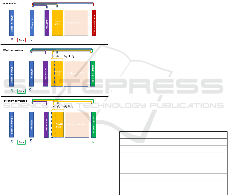
Figure 1: Phenotypes generating mechanism. The

phenotypes were generated using patients’ age, gender,

SNP genotypes, and an environmental factor or a related

diagnosis status. The top solid arrows represent the true

phenotype generating mechanism. In the independent

model, all factors were independently associated with the

phenotype. In the weakly correlated model, the related

diagnosis and the phenotype shared a subset of causal

SNPs, but the associations 



and 



were independent. In

the strongly correlated model, the subset of shared casual

SNPs had the same associations, as in



is a subset of 



The bottom dotted arrows indicate the phenotype error

generating mechanism. The biased phenotypes were

generated based on the values of the true phenotype and the

environmental factor or the related diagnosis.

Furthermore, cardiac arrest is also associated with

heart failure diagnosis. In this study, this model was

named strongly correlated model. The SNPs in all

models were randomly selected from the common

SNPs (minor allele frequency > 5%) in the eMERGE

EHR genetic data. The mathematical models for the

phenotype simulation are presented in the following

sections.

2.2.1 Independent Model

In this model, the phenotype Y was generated through

the logistic model.

Phenotype:

Logit



PY  1



~30.3∗Age0.1∗Gender

∑



∗







2∗_

The coefficients for the intercept, age, gender, and

environmental factors (Env_factor) were selected so

that the disease prevalence was around 30%. The

same coefficients were also used for the weakly

correlated and the strongly correlated model so that

the models were comparable. The distributions of the

random variables in all equations were listed in Table

2.2.2 Weakly Correlated Model

In the weakly correlated model, a related diagnosis

was first generated using q SNPs, where q was a

subset of p SNPs that were used to generate the

phenotype. In addition, the coefficients  for

generating the related diagnosis were independent of

β that were used to generate the phenotype.

Table 1: Parameter values for phenotype simulation.

Variable Value

Total randomly selected SNPs 500

Phenotype associated SNPs p = 100

Diagnosis associated SNPs q = 50

Age Normal (40, 10)

Gender Bernoulli (p = 0.5)

Environmental factor (Env_factor) Bernoulli (p = 0.5)

Phenotype ~ SNP associations

 ~ Normal (0, 0.3)

Related diagnosis ~ SNP associations

 ~ Normal (0, 0.3)

Related diagnosis:

Logit



PRelateddiagnosis  1



~



∗







;q⊆

Phenotype:

Logit



PY  1



~ 3  0.3∗Age0.1∗Gender

∑



∗







2∗ 

Evaluation of Phenotyping Errors on Polygenic Risk Score Predictions

125

2.2.3 Strongly Correlated Model

The strongly correlated model was the same as the

weakly correlated model except that the related

diagnosis and the phenotype shared a subset of q

SNPs as well as their coefficients.

Related diagnosis:

LogitPRelateddiagnosis  1~

∑



∗



;q ⊆





;



⊆





Phenotype:

Logit



Y1



~30.3∗Age0.1∗Gender

∑



∗









2∗ 

2.3 Biased Phenotype Due to Errors

As shown in Figure 1, the biased phenotypes were

generated based on the value of the true phenotypes

as well as the environmental factor or the related

diagnosis (Figure 1, dotted arrows at the bottom). The

intuition was that, first, the biased phenotype would

be expected to be a deviation from the true phenotype.

Second, many of the phenotyping algorithms utilized

by EHR systems used environmental and diagnosis

variables to determine the phenotype or disease

status, thus, the precision of the phenotype was also

associated with these factors (Kirby et al., 2016;

Robinson, Wei, Roden, & Denny, 2018; Wei &

Denny, 2015). Mathematically, the phenotyping

errors were determined by the sensitivity and

specificity:

 



  

 



 

Sensitivity and specificity measures how close the

biased phenotype is to the true phenotype. As an

example,

in the independent model, the biased

phenotype was generated using the following 2x2

tables. The 2x2 table shows that the biasness of the

phenotype depends on both the phenotype as well as

an environmental factor. Thus, there were two pairs

of sensitivity and specificity values for the two

variables.

 Y=1 Y=0

ENV_FACTOR=1 Sensitivity

Exposure

 Specificity

Exposure



ENV_FACTOR=0 Sensitivity

non_Exposure

 Specificity

non_Exposure



Mathmatically, the Sensitivity

Exposure

controlled

the sensitivity of the biased Y when the true

phenotype Y = 1 and Env_factor = 1. The new

phenotype value under this combination was

generated using the Bernoulli distribution with the

probability equaled to

Sensitivity

Exposure

. In contrast,

the

Specificity

Exposure

determined the probably of the

biased Y = 0, when true Y = 0 and the Env_factor =

0. The value was generated by Bernoulli (1-

Specificity

Exposure

). Thus, the degree of phenotyping

errors was controlled by the values of the sensitivity

of specificity. As a special case, a phenotype was the

gold standard when sensitivity = specificity = 100%.

For biased phenotypes, the phenotyping error was

non-differential when the sensitivities (e.g. a) and

specificities (e.g. b) were the same across the two

Env_factor levels; otherwise, the error was

differential (e.g. a, b, c, and d). For instance, a

phenotype that is more error-prone for patients with

lower levels of environmental exposure would be

differentially biased.

NON‐DIFFERENTIALPHENOTYPINGERROR

 Y=1 Y=0

ENV_FACTOR=1 a% b%

ENV_FACTOR=0 a% b%

DIFFERENTIALPHENOTYPINGERROR

 Y=1 Y=0

ENV_FACTOR=1 a% c%

ENV_FACTOR=0 b% d%

2.4 Biased Phenotype Generation

For all phenotypes (independent, weakly correlated,

and strongly correlated), a range of phenotyping

errors were introduced using different levels of

sensitivity and specificity. In addition, differential

and non-differential error generating mechanisms

were applied at each sensitivity and specificity level.

To simplify the presentation of the results, the same

value of sensitivity and specificity for the non-

differential phenotyping error was used (Table 2). For

differential phenotyping error, one sensitivity and one

specificity were kept at 99%, while the others varied

(Table3). Overall, 60 biased phenotypes were

generated.

2.5 Evaluation of PRS Prediction

The effect of the phenotyping errors on PRS

prediction was evaluated in the following steps.

1. Split the data into training and testing

2. Sample sizes of the data split

BIOINFORMATICS 2020 - 11th International Conference on Bioinformatics Models, Methods and Algorithms

126

3. Obtain coefficients for the SNPs using the

training data

4. Construct PRSs in both training and testing data

5. Build a predictive model using the PRS in the

training data

6. Apply the model to the test data

7. Compare the predicted phenotype value to the

true phenotype value

The data was split into the training and testing

datasets, with the testing dataset being held out for

evaluation. Using the training data, all SNPs’

marginal association, β



,

, with the biased

phenotypes were obtained. The marginal associations

from the training data were then used to construct

PRSs in both the training and testing data. Next, a

predictive model was built using the PRS in the

training data; the model was subsequently applied to

the testing PRS to obtain the predicted phenotype.

The predicted phenotype was compared with the true

phenotype in the testing data to obtain the testing

area-under-the-curve (AUC) value. The entire

process, from phenotype simulation to PRS

prediction, was repeated 100 times using different

random seeds to obtain 100 replications of the results.

3 RESULT

In all simulations, gold standard results were included

to serve as the baselines for comparison. The gold

standards demonstrated the maximum obtainable

prediction accuracies from PRSs that were generated

using the true phenotype. Figure 1 showed a change

in PRS prediction accuracy as more non-differential

errors were added into the phenotype. The accuracies

gradually decreased from gold standard to 50%

sensitivity and specificity. At 50% sensitivity and

specificity, the biased phenotype was generated the

same way as coin-flipping. Thus, the prediction

accuracies of PRS at this error level was also around

50%. Notably, the gold standard accuracies were also

different even when the simulation parameter values

were the same for all three phenotypes.

4 DISCUSSION

Disease risk prediction utilizing genetic information

via PRS has shown great promise in many complex

human diseases. With the increasing availability of

linked genetic data in EHR systems, PRS prediction

can be widely applied to many phenotypes and

diseases to identify high-risk patients for better

disease prevention and treatment care. Nevertheless,

patients’ true disease statuses are often unknown.

Thus, the observed disease status is only a proxy for

the true disease status, and the observed status will be

biased due to phenotyping errors. In this study, we

quantified the degradation of PRS prediction using

three different types of phenotype under the

differential and non-differential phenotyping errors.

Table 2: Sensitivity and specificity for the non-differential phenotyping error.

Error model name Error mechanism

Gold standard No error

X = (95, 90, 85, 80, 75, 70,

65, 60, 55, 50)

 Y=1 Y=0

Env_factororDiagnosis=1

Sensitivity=X% Specificity=X%

Env_factororDiagnosis=0

Sensitivity=X% Specificity=X%

Table 3: Sensitivity and specificity for the non-differential phenotyping error.

Error model name Error mechanism

Gold standard No error

X = (95, 90, 85, 80, 75, 70,

65, 60, 55, 50)

 Y=1 Y=0

Env_factororDiagnosis=1

Sensitivity=X% Specificity=99%

Env_factororDiagnosis=0

Sensitivity=99% Specificity=X%

Evaluation of Phenotyping Errors on Polygenic Risk Score Predictions

127

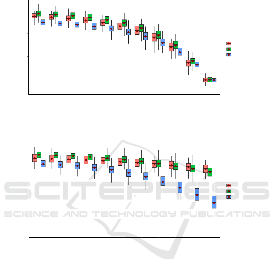
Figure 2: Performance of PRS prediction under non-differential phenotyping error. Each boxplot represents 100 replications

of the same experiment using different datasets. The x-axis indicates the sensitivity and specificity level set by variable X in

table 2. The y-axis shows the prediction AUC on the testing data.

Figure 3: Performance of PRS prediction under differential phenotyping error. Each boxplot represents 100 replications of

the same experiment using different datasets. The x-axis indicates the sensitivity and specificity level set by variable X in

table 3. The y-axis shows the prediction AUC on the testing data.

We utilized the eMERGE EHR genetic data so

that the SNPs had the minor allele frequency

distribution and correlation structure that are

observed in the real patients’ data. Using the SNPs

data along with other demographic and clinical

variables, we simulated three different phenotypes

with increasing levels of complexity (Figure 1). For

the phenotype generated under the independent

model, all variables independently related to the

phenotype. Here, we assumed that an individual’s

genetic factors do not affect one’s environmental

exposure. Under the weakly correlated model, we

used a related diagnosis status to determine the

phenotype status, and the two were associated with a

common subset of SNPs through pleiotropic effects.

In this case, we assumed that the associated effects

were different between the related diagnosis and the

phenotype. This is likely when the phenotypes are

regulated through different biological mechanisms,

such as between heart diseases and mental disorders

(Andreassen et al., 2013; Li, Duan, et al., 2019; X.

Zhang et al., 2019). Finally, in the strongly correlated

model, the diagnosis and the phenotype were assumed

to be more similar due to the shared underlying SNPs

as well as their coefficients. This reflects a possible

scenario when a subtype of disease is used to

diagnose the main disease.

●

0.747

0.786

0.773

0.743

0.781

0.769

0.737

0.775

0.764

0.73

0.769

0.756

0.72

0.758

0.746

0.706

0.744

0.731

0.687

0.722

0.711

0.659

0.691

0.682

0.619

0.648

0.64

0.565

0.58

0.573

0.499

0.5

0.501

0.5

0.6

0.7

0.8

Testing AUC

Simulation model

Independent

Weakly correlated

Strongly correlated

●

0.748

0.785

0.772

0.745

0.783

0.769

0.74

0.78

0.767

0.734

0.776

0.764

0.725

0.772

0.761

0.713

0.765

0.758

0.697

0.759

0.753

0.677

0.75

0.749

0.653

0.74

0.743

0.624

0.728

0.736

0.593

0.716

0.728

0.5

0.6

0.7

0.8

Te s t i n g AU C

Simulation model

Independent

Weakly correlated

Strongly correlated

BIOINFORMATICS 2020 - 11th International Conference on Bioinformatics Models, Methods and Algorithms

128

As expected, as more phenotyping errors were

added to the three phenotypes, the prediction

accuracy of PRS decreased. However, the rates of the

decrease depended on the type of phenotyping errors.

First, the gold standards’ accuracy in Figure 2 and

Figure 3 were similar because they both represented

PRS predictive power without any phenotyping

errors. Interestingly, the PRS achieved the best

performance in the phenotype generated from the

weakly correlated model, followed by the

independent and strongly correlated model. This can

be explained by the different amount of genetic

contribution to the phenotype. In the weakly

correlated model, SNPs contributed to the phenotype

through two mechanisms: 1. direct associations with

the phenotype. 2. Indirect associations through the

related diagnosis. Because the indirect associations

were independent of the direct associations, the SNPs

contributed “twice” to the phenotype. In contrast, in

the independent model, the SNPs were only

associated with the phenotype through their direct

associations. And in the strongly correlated model,

the SNPs’ associations were diminished because part

of the associations was mediated by the related

diagnosis. Second, non-differential phenotyping

errors similarly affected all phenotypes. The relative

order of PRS prediction accuracies did not change as

more non-differential phenotyping errors were added.

Finally, differential phenotyping errors, which are

more likely to be observed in real data, exhibited

different accuracy trajectories for the phenotypes.

The independent model was affected the least, likely

because the SNPs and the environmental factor were

independent. Thus, differential phenotyping errors

induced by the environmental factor did not have a

major impact on the PRS prediction accuracy.

However, in the weakly correlated and strongly

correlated model, both the phenotype and the related

diagnosis were associated with the SNPs. Thus,

differential errors based on these variables had a

severe impact on the PRS, with the strongest impact

in the strongly correlated model. In summary, non-

differential phenotyping errors affected PRS

prediction equally among the phenotypes.

Differential phenotyping errors had an increased

impact on PRS prediction if the target phenotype and

the variables used to determine the phenotype have a

shared genetic component.

While it is useful to understand the impact of

phenotyping errors on PRS prediction, it is also

important to identify approaches that can minimize

the error. One effective approach to reducing error is

through manual chart review of patients’

comprehensive clinical histories by doctors or

domain experts. However, manual review is both

time-consuming and expensive. A potential

alternative approach is to chart review a subset of

patients to determine the amount of phenotyping error

as well as the error mechanism. Then, the results

presented in this study could serve as a guideline to

determine whether the errors are within the

acceptable range. If not, the phenotype quality needs

to be improved. For future studies, the impact of

phenotyping errors on the continuous outcome can be

explored. Furthermore, phenotype differences across

individuals or populations depend on both genetic and

environmental factors(Rosenberg, Edge, Pritchard, &

Feldman, 2019). To evaluate the relative importance

of these factors, it is essential to verify the accuracies

of the measurements. Thus, more complex error

patterns that depend on multiple environmental or

clinical variables are likely to be more realistic and

should be investigated. Finally, AUC is the current

standard measurement for PRS performance.

However, some studies suggested that AUC may not

be the best metric for evaluating classification

accuracy. Thus, other accuracy metrics, such as net

reclassification improvement or integrated

discrimination improvement can be used (Pencina,

D’Agostino, D’Agostino, & Vasan, 2008).

REFERENCES

Andreassen, O. A., Djurovic, S., Thompson, W. K., Schork,

A. J., Kendler, K. S., O’Donovan, M. C., … Dale, A.

M. (2013). Improved detection of common variants

associated with schizophrenia by leveraging pleiotropy

with cardiovascular-disease risk factors. American

Journal of Human Genetics, 92(2), 197–209.

https://doi.org/10.1016/j.ajhg.2013.01.001

Chen, Y., Wang, J., Chubak, J., & Hubbard, R. A. (2019).

Inflation of type I error rates due to differential

misclassification in EHR-derived outcomes: Empirical

illustration using breast cancer recurrence.

Pharmacoepidemiology and Drug Safety, 28(2), 264–

268. https://doi.org/10.1002/pds.4680

Duan, R., Cao, M., Wu, Y., Huang, J., Denny, J. C., Xu, H.,

& Chen, Y. (2016). An Empirical Study for Impacts of

Measurement Errors on EHR based Association

Studies. AMIA ... Annual Symposium Proceedings.

AMIA Symposium, 2016, 1764–1773. Retrieved from

http://www.ncbi.nlm.nih.gov/pubmed/28269935

Euesden, J., Lewis, C. M., & O’Reilly, P. F. (2015).

PRSice: Polygenic Risk Score software.

Bioinformatics, 31(9), 1466–1468. https://doi.org/

10.1093/bioinformatics/btu848

Khera, A. V., Chaffin, M., Wade, K. H., Zahid, S.,

Brancale, J., Xia, R., … Kathiresan, S. (2019).

Polygenic Prediction of Weight and Obesity

Evaluation of Phenotyping Errors on Polygenic Risk Score Predictions

129

Trajectories from Birth to Adulthood. Cell, 177(3),

587-596.e9. https://doi.org/10.1016/j.cell.2019.03.028

Khera, A. V, Chaffin, M., Aragam, K. G., Haas, M. E.,

Roselli, C., Choi, S. H., … Kathiresan, S. (2018).

Genome-wide polygenic scores for common diseases

identify individuals with risk equivalent to monogenic

mutations. Nature Genetics, 50(9), 1219–1224.

https://doi.org/10.1038/s41588-018-0183-z

Kirby, J. C., Speltz, P., Rasmussen, L. V, Basford, M.,

Gottesman, O., Peissig, P. L., … Denny, J. C. (2016).

PheKB: a catalog and workflow for creating electronic

phenotype algorithms for transportability. Journal of

the American Medical Informatics Association, 23(6),

1046–1052. https://doi.org/10.1093/jamia/ocv202

Li, R., Chen, Y., & Moore, J. H. (2019). Integration of

genetic and clinical information to improve imputation

of data missing from electronic health records. Journal

of the American Medical Informatics Association.

https://doi.org/10.1093/jamia/ocz041

Li, R., Duan, R., Kember, R. L., Rader, D. J., Damrauer, S.

M., Moore, J. H., & Chen, Y. (2019). A regression

framework to uncover pleiotropy in large-scale

electronic health record data. Journal of the American

Medical Informatics Association. https://doi.org/

10.1093/jamia/ocz084

Lo, A., Chernoff, H., Zheng, T., & Lo, S.-H. (2015). Why

significant variables aren’t automatically good

predictors. Proceedings of the National Academy of

Sciences of the United States of America, 112(45),

13892–13897. https://doi.org/10.1073/pnas.151828

5112.

Manolio, T. A., Collins, F. S., Cox, N. J., Goldstein, D. B.,

Hindorff, L. A., Hunter, D. J., … Visscher, P. M.

(2009). Finding the missing heritability of complex

diseases. Nature, 461(7265), 747–753. https://doi.org/

10.1038/nature08494

Martin, A. R., Gignoux, C. R., Walters, R. K., Wojcik, G.

L., Neale, B. M., Gravel, S., … Kenny, E. E. (2017).

Human Demographic History Impacts Genetic Risk

Prediction across Diverse Populations. The American

Journal of Human Genetics, 100(4), 635–649.

https://doi.org/10.1016/j.ajhg.2017.03.004

Martin, A. R., Kanai, M., Kamatani, Y., Okada, Y., Neale,

B. M., & Daly, M. J. (2019). Current clinical use of

polygenic scores will risk exacerbating health

disparities. BioRxiv, 441261. https://doi.org/10.1101/

441261

McCarty, C. A., Chisholm, R. L., Chute, C. G., Kullo, I. J.,

Jarvik, G. P., Larson, E. B., … eMERGE Team. (2011).

The eMERGE Network: a consortium of

biorepositories linked to electronic medical records

data for conducting genomic studies. BMC Medical

Genomics, 4, 13. https://doi.org/10.1186/1755-8794-4-

Pencina, M. J., D’Agostino, R. B., D’Agostino, R. B., &

Vasan, R. S. (2008). Evaluating the added predictive

ability of a new marker: From area under the ROC

curve to reclassification and beyond. Statistics in

Medicine, 27(2), 157–172. https://doi.org/10.1002/

sim.2929

Purcell, S. M., Wray, N. R., Stone, J. L., Visscher, P. M.,

O’Donovan, M. C., Sullivan, P. F., … Sklar, P. (2009).

Common polygenic variation contributes to risk of

schizophrenia and bipolar disorder. Nature, 460(7256),

748. https://doi.org/10.1038/nature08185

Robinson, J. R., Wei, W.-Q., Roden, D. M., & Denny, J. C.

(2018). Defining Phenotypes from Clinical Data to

Drive Genomic Research.

https://doi.org/10.1146/annurev-biodatasci

Rosenberg, N. A., Edge, M. D., Pritchard, J. K., & Feldman,

M. W. (2019). Interpreting polygenic scores, polygenic

adaptation, and human phenotypic differences.

Evolution, Medicine, and Public Health, 2019(1), 26–

34. https://doi.org/10.1093/emph/eoy036

Schizophrenia Working Group of the Psychiatric Genomics

Consortium. (2014). Biological insights from 108

schizophrenia-associated genetic loci. Nature,

511(7510), 421–427. https://doi.org/10.1038/

nature13595

Torkamani, A., Wineinger, N. E., & Topol, E. J. (2018).

The personal and clinical utility of polygenic risk

scores. Nature Reviews Genetics, 19(9), 581–590.

https://doi.org/10.1038/s41576-018-0018-x

Verma, S. S., de Andrade, M., Tromp, G., Kuivaniemi, H.,

Pugh, E., Namjou-Khales, B., … Ritchie, M. D. (2014).

Imputation and quality control steps for combining

multiple genome-wide datasets. Frontiers in Genetics,

5, 370. https://doi.org/10.3389/fgene.2014.00370

Visscher, P. M., Wray, N. R., Zhang, Q., Sklar, P.,

McCarthy, M. I., Brown, M. A., & Yang, J. (2017). 10

Years of GWAS Discovery: Biology, Function, and

Translation. The American Journal of Human Genetics,

101(1), 5–22. https://doi.org/10.1016/J.AJHG.2017.

06.005

Wei, W.-Q., & Denny, J. C. (2015). Extracting research-

quality phenotypes from electronic health records to

support precision medicine. Genome Medicine, 7(1),

41. https://doi.org/10.1186/s13073-015-0166-y

Yang, J., Benyamin, B., McEvoy, B. P., Gordon, S.,

Henders, A. K., Nyholt, D. R., … Visscher, P. M.

(2010). Common SNPs explain a large proportion of the

heritability for human height. Nature Genetics, 42(7),

565–569. https://doi.org/10.1038/ng.608

Zhang, J.-P., Robinson, D., Yu, J., Gallego, J.,

Fleischhacker, W. W., Kahn, R. S., … Lencz, T. (2019).

Schizophrenia Polygenic Risk Score as a Predictor of

Antipsychotic Efficacy in First-Episode Psychosis.

American Journal of Psychiatry, 176(1), 21–28.

https://doi.org/10.1176/appi.ajp.2018.17121363

Zhang, X., Veturi, Y., Verma, S., Bone, W., Verma, A.,

Lucas, A., … Ritchie, M. D. (2019). Detecting potential

pleiotropy across cardiovascular and neurological

diseases using univariate, bivariate, and multivariate

methods on 43,870 individuals from the eMERGE

network. Pacific Symposium on Biocomputing. Pacific

Symposium on Biocomputing, 24, 272–283. Retrieved

from http://www.ncbi.nlm.nih.gov/pubmed/30864329

BIOINFORMATICS 2020 - 11th International Conference on Bioinformatics Models, Methods and Algorithms

130