
Extraction of Intrinsic Fluorescence in Fluorescence Imaging of
Turbid Tissues
Gennadi Saiko
1a
and Alexandre Douplik
2b
1
Swift Medical Inc, 1 Richmond St W, Toronto, Canada
2
Department of Physics, Ryerson University, Toronto, Canada
Keywords: Fluorescence, Fluorescence Imaging, Intrinsic Fluorescence, Turbid Tissues.
Abstract: Interpretation of tissue fluorescence spectra can be complicated due to interplay with tissue optics. We have
developed a photon propagation approach for correction of fluorescence on absorption in two realistic
scenarios: when fluorophores are located a) on the surface of the turbid tissue and b) in a layer inside the
turbid tissue. The approach takes into account the diffuse reflection of the tissue at excitation and emission
wavelengths and does not require any precise measurement of optical properties (e.g., coefficient of
absorption). The approach can be implemented using an inexpensive imaging setup and can be used in any
setting.
1 INTRODUCTION
Fluorescence imaging is an important optical clinical
modality and has numerous applications in
diagnostics and surgical guidance.
Advances in clinical fluorescence imaging are
related mostly to fluorescence angiography, which is
based on the injection of a fluorescent dye in the
bloodstream and subsequent visualization of blood
vessels. Initially, the method was developed for
ophthalmology using fluorescein as the dye (e.g.,
Intravenous Fluorescein Angiography (IVFA) or
Fluorescent Angiography (FAG) for examining the
circulation of the retina and choroid).
Recently, the method has been extended to other
blood vessels using Indocyanine green (ICG), which
is a non-toxic, protein-bound dye that is retained
within the vasculature after intravenous injection for
several minutes until rapid clearance by the liver
(Sevick-Muraca, 2012).
Endogenous fluorescence in tissues is associated
with tissues’ autofluorescence and bacterial (or
fungal) presence.
Autofluorescence in turbid tissues is attributed
mainly to proteins, collagen, and elastin. Collagen (or
elastin in other tissues) is the major contributor to the
a
https://orcid.org/ 0000-0002-5697-7609
b
https://orcid.org/ 0000-0001-9948-9472
tissue autofluorescence; it is accountable for up to
95% of fluorescence in visible spectra.
Collagen/elastin is excited in the range of 370-450 nm
and re-emits in the range 490-580 nm.
Some interesting possibilities are connected with
other tissue fluorophores, including the reduced form
of coenzyme nicotinamide adenine dinucleotide
(NADH), which is sensitive to tissue oxygen
concentration.
Bacteria fluorescence can be particularly
important in wound care to a) identify particular
strains in the wound, b) assess (qualitatively or
quantitatively) bacteria presence, or c) guide
sampling, debridement, or antimicrobial selection.
All wounds contain bacteria (e.g., Staphylococcus,
Streptococcus, Pseudomonas species, and Coliform
bacteria), at levels ranging from contamination
through critical colonization to infection. Most of the
clinically important strains (both gram-positive and
negative) clearly show a distinctive double-peak of
tryptophan fluorescence (Dartnell, 2013).
Unfortunately, these bands are within the UVC band,
which makes it problematic for clinical use. However,
some clinically relevant bacteria (S. aureus, S.
epidermidis, Candida, S. marcescens, Viridans
streptococci, Corynebacterium diphtheriae, S.
pyogenes, Enterobacter, and Enterococcus) produces
Saiko, G. and Douplik, A.
Extraction of Intrinsic Fluorescence in Fluorescence Imaging of Turbid Tissues.
DOI: 10.5220/0008919401230129
In Proceedings of the 13th International Joint Conference on Biomedical Engineering Systems and Technologies (BIOSTEC 2020) - Volume 2: BIOIMAGING, pages 123-129
ISBN: 978-989-758-398-8; ISSN: 2184-4305
Copyright
c
2022 by SCITEPRESS – Science and Technology Publications, Lda. All rights reserved
123
red fluorescence (Kjeldstad, 1985), while P.
aeruginosa produced a bluish-green fluorescence
(Cody, 1987).
Interpretation of tissue fluorescence spectra could
be complicated due to interplay with tissue optics.
Thus, fluorescence spectra measured in vivo can be
significantly different from those from pure
fluorophores in lab conditions.
Several approaches to deal with this problem have
been developed in recent years. Comprehensive
review of correction techniques was performed by
Bradley et al (Bradley, 2006). They classified these
techniques into four broad groups: empirical
techniques, measurement-method based techniques,
theory based techniques, and Monte Carlo based
techniques. In particular, some groups (Liu 1992,
Anidjar 1996) used spectroscopy at several
wavelengths (e.g., their ratio) to take into account
absorption. Other groups attempted to retrieve
intrinsic fluorescence spectra from raw fluorescence
spectra measured in biological tissues. In particular,
Wu et al. (Wu, 1993) developed a photon migration
model to extract intrinsic fluorescence in turbid
media. An amended photon migration model was
proposed by Muller et al. (Muller, 2001). Pfefer et al.
(Pfefer, 2001) used Monte Carlo simulations to
analyze the effect of optical fiber diameter, distance
to tissue, and numerical aperture on light propagation
during fluorescence spectroscopy with a single-fiber
probe. Kim et al. (Kim, 2010) proposed an elegant
model to quantify in vivo fluorescence in spatially
resolved fiber optic measurements. Valdes et al.
(Valdes, 2017) successfully applied Kim’s model to
retrieve intrinsic fluorescence in an imaging
modality. Yang et al. (Yang, 2014) applied structured
light to decrease the influence of absorption on
fluorescence imaging. Lin et al. (Lin, 2001) compared
fluorescence and reflection spectra to reduce spectral
distortions caused by superficial blood contamination
on tissue optical spectra during surgical operations
(resections). More recently Zhang et al (Zhang, 2018)
used particle swarm optimization algorithm in
combination with a optic fiber probe to extract
intrinsic tissue fluorescence spectrum.
However, existing models suffer from several
shortcomings, which complicate their translation into
clinical imaging applications. Namely, some of them
(e.g., Pfefer, 2001) were developed for a particular
collection geometry (e,g, a single fiber or multi-fiber
geometry), which are quite different from imaging
geometries. Other (e.g., Kim, 2010) require accurate
measurements of optical tissue parameters (e.g., the
absorption coefficient), which can be impractical in
non-hospital applications.
The purpose of this article is to develop an
approach, which can deconvolute intrinsic
fluorescence in typical tissue imaging geometry
without precise measurements of optical tissue
parameters. Such as fluorescence imaging has
multiple applications in wound care, we will illustrate
our approach with fluorophores produced by
clinically relevant bacteria (P.aeruginosa and
S.aureus). It is a particularly complicated case,
because these fluorophores (pyoverdine and
porphyrins, respectively) have absorption peaks in the
same range (400nm) as hemoglobins.
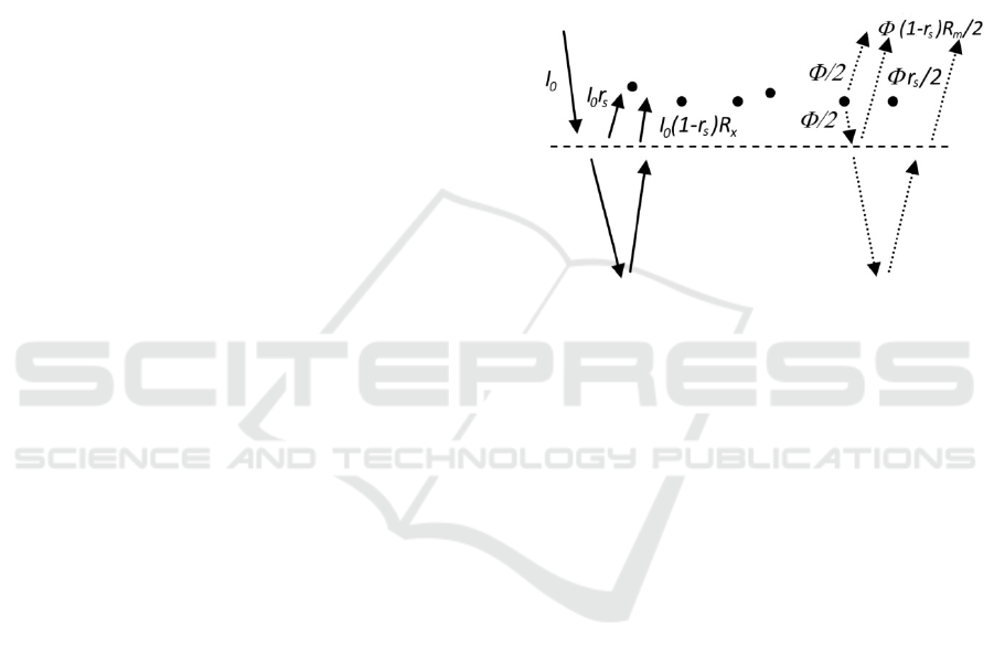
Figure 1: Contributions to the excitation flux (left side, solid
lines) and the emission flux (right side, dotted lines) if
fluorophores are located above the surface.
The article is structured as follows:
First, we develop a photon propagation approach
to calculate the fluorescence if fluorophores are
located on the surface of the tissue. For this, we
consider excitation and emission photons separately.
Then, we will use a similar photon propagation
approach to calculate the fluorescence if fluorophores
are located inside the tissue.
2 THEORY
In realistic conditions, biological fluorophores are
typically located inside the tissue (e.g., collagen).
However, in some cases, fluorophores can be located
on the surface of the tissue (e.g., bacteria and fungi
during contamination and colonization stages). So, to
elucidate the differences between these two cases, we
consider them separately.
2.1 Fluorophores on the Surface
Let’s consider fluorophores that are located on the
surface of the tissue.
BIOIMAGING 2020 - 7th International Conference on Bioimaging
124
The fluorescence output (flux, W/m
2
)
is
proportional to the surface density of fluorophores n,
their absorption cross-section
and quantum yield
,
and an excitation flux I
x
.
Φ=
=
(1)
here f is an intrinsic fluorescence.
The excitation flux I
x
(see Figure 1), consists of an
inbound directional flux I
0
(illumination) and
outbound directional flux I
r
, which was reflected from
the tissue. The outbound flux I
r
consists of two
components: specular reflection I
s
and diffuse
reflectance I
d
. If we assume that the absorption on the
surface is small, then we can write
=
+
+
=
(1 +
+(1−
)
)
(2)
here, r
s
is the coefficient of specular reflection (
=
( − 1)
/( + 1)
, where n is the relative index of
refraction), and R
x
is the coefficient of diffuse
reflectance of the tissue at an excitation wavelength.
The fluorophores re-emit isotropically in all
directions (see Figure 1). Thus, ½ of the output goes
into the upper semisphere and can be immediately
collected by the imaging system. The other half of the
fluorescence output will shine into the lower
semisphere. A minor part of it will be immediately
reflected by the surface (specular reflection), while
the major part will go into the tissue, and some of
them will be reflected through diffuse reflectance.
Thus, the measured fluorescence can be written as
=Φ/2(1+
+(1−
)
)
(3)
here, R
m
is the coefficient of diffuse reflectance of the
tissue at an emission wavelength.
It should be noted that (3) assumes that we can
collect all photons emitted in the upper semisphere,
which is not true in any realistic imaging scenario. A
realistic fluorescence signal will contain a geometric
factor, which takes into account a collection geometry
(e.g., numeric aperture). However, such as the
collection geometry stays constant in the experiment
we will ignore this geometric factor in our
calculations.
Then, the intrinsic fluorescence f can be expressed
as
=
2
1
(
1+
+
(
1−
)
)
∗
1
(
1+
+
(
1−
)
)
(4)
Thus, the correction factor contains the coefficient
of specular reflection and coefficients of tissue
reflectance at excitation and emission wavelengths.
2.2 Fluorophores in the Tissue
The more realistic fluorescence imaging scenario is
when fluorophores are located in the tissue. It can be
collagen, which is localized mostly in the dermis,
siderophores, or metabolic by products produced by
bacteria in the epidermis (impetigo), dermis
(folliculitis, erysipelas), subcutaneous fat (cellulitis)
or fascia (necrotic fasciitis). It can be noted that in all
of the mentioned above cases, the fluorophores are
localized in a layer (e.g., collagen in interstitial
tissue), rather homogeneously distributed across
depth. Based on this observation, the following model
can be considered: the fluorophores are located in a
thin layer parallel to the tissue surface. In this case we
can ignore the heterogeneity of excitation light
distribution within this layer.
To calculate the fluorescence signal, we can take
the following approach: 1) calculate the excitation
flow in the tissue, 2) multiply it by the intrinsic
fluorescence, and 3) take into account reflection and
scattering of the emission flux within the tissue using
emission photon propagation model.
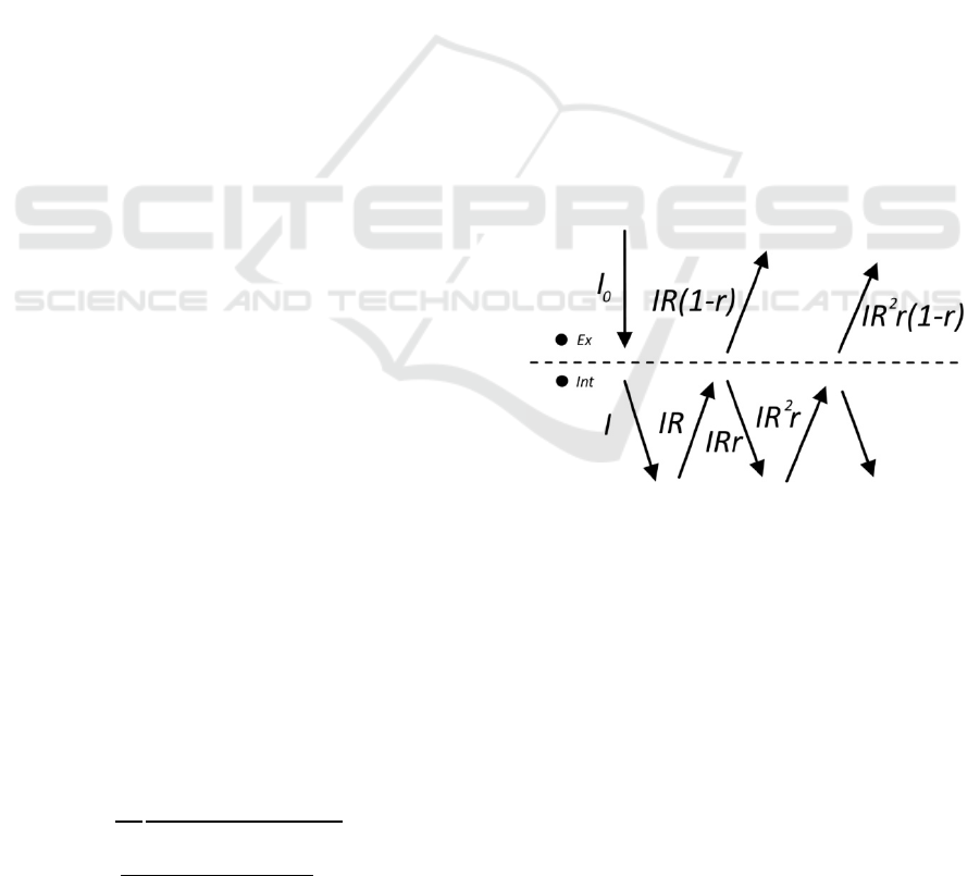
Figure 2: Contributions to the excitation flux.
The fluorophores absorb photons from the
incoming (e.g. collimated) flow. However, in
addition to the incoming flow, they will be excited by
a flow of diffusively reflected photons. Their steady-
state distribution will be greatly impacted by the
optical properties of the tissue and particularly by
mismatched boundary conditions. To take into
account that diffuse flow we can consider the
following simplified model. Let’s consider two points
in the close vicinity of the interface: one is slightly
above, one is slightly below the surface (see Figure
2). We can roughly calculate the flow in each of these
points using the following considerations. Let’s
assume that the incoming flux in the tissue is I (=
Extraction of Intrinsic Fluorescence in Fluorescence Imaging of Turbid Tissues
125
(1 −
)). The inbound flux has the probability R
(bulk tissue reflectance) to be diffusively reflected.
Thus, the diffusively reflected flow (outbound flux)
near the surface will be IR. Now, on the surface, the
light can be reflected with the probability r (specular
reflection coefficient, which depends solely on the
relative index of refraction) or escape the tissue with
probability 1-r. And this process is repeated
indefinitely.
Thus, the flow just below the surface can be
calculated as
=+++
+⋯
=
1−
+
1−
(5)
The flow just above the surface can be calculated
as
=
(
1−
)
+
(
1−
)
+⋯
=
(1 − )
1−
(6)
From (6) one can see that
=
, where
=
(1 − )
1−
(7)
is the diffuse reflectance of the tissue, which can be
measured experimentally.
According to (5), the flow just below the surface
is times larger than the initial inbound flow I (
=
), where
=
1+
1−
(8)
Such as the probability R is unknown, we can
express it using diffuse reflectance R
d
, which can be
measured experimentally and r, which can be
assessed analytically or numerically. Resolving (7)
over R and substituting it into (8) gives us
=1+
+
2
1−
(9)
Specular reflection coefficient r can be found
using Fresnel theory and assumptions about angular
light distribution below the surface (Welch, 2011).
The simplified diffuse approximation model (Star,
2011) provides a good estimate for that value; =
1−
, where n is the relative index of refraction. In
this case, (9) can be rewritten as
~1 + (2
−1)
(9’)
For a realistic index of refraction n=1.41, one can
see that ~1 + 3
, which is in a reasonable
agreement with estimates based on diffuse
approximation theory (Star, 2011).
Now, let’s turn to the fluorescence. Excitation
photons propagate through a thin fluorescent layer in
a ballistic way. Thus, the probability of getting
absorbed is = , where N is the volume
concentration of fluorophores, l is the thickness of
their layer. Then, the fluorophores re-emit light with
probability
(quantum yield) isotropically in all
directions (see Figure 3).
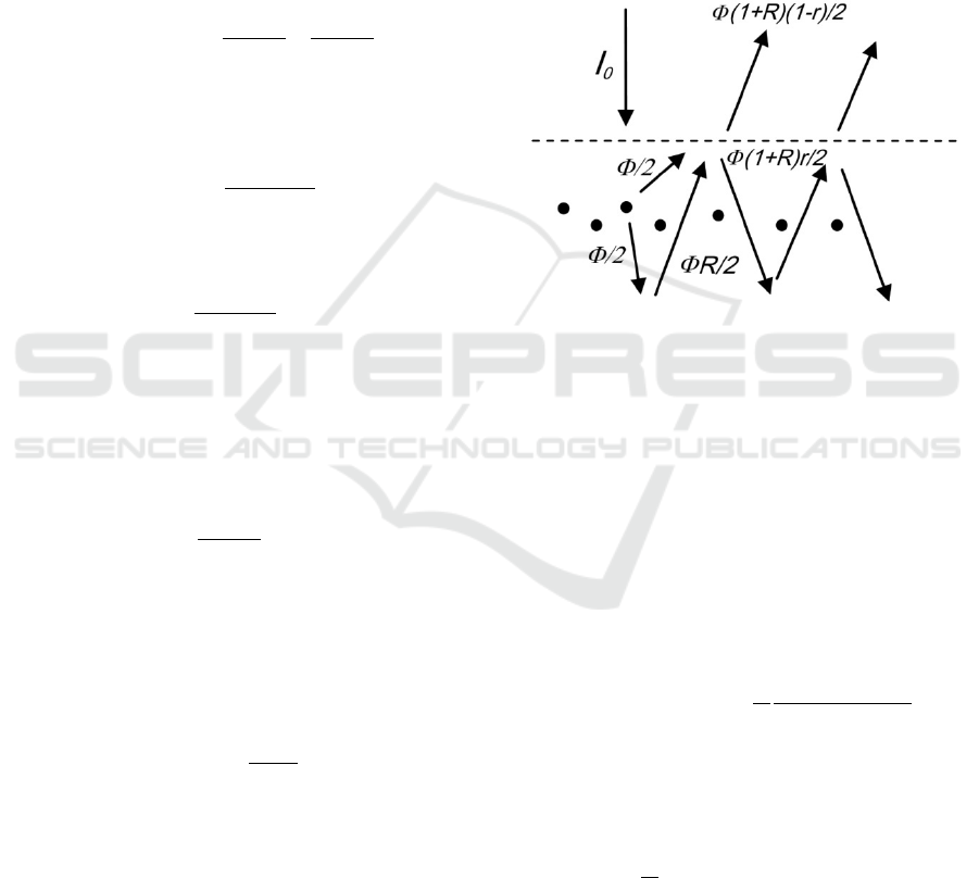
Figure 3: Contributions to the emission flux if fluorophores
are located below the surface.
Thus, ½ of the output is emitted in the upper
semisphere. The other half of the fluorescence output
will shine in the lower semisphere, and some of these
photons will be reflected through diffuse reflectance
with probability R. Similarly to (6), if we take into
account the probability of specular reflection on the
tissue/air interface r, then the measured fluorescence
can be calculated as
=Φ
(
1+
)(
1−
)
/2
+Φ
(
1+
)
(
1−
)
/2
+⋯=
Φ
2
(1 + )(1 − )
1−
(10)
One can see that a multiplier in (10) is equal to
(1 − ) . Thus, using (9) this expression can be
rewritten as:
=
Φ
2
(1 +
−+
)
(11)
here, R
d
should be measured at the emission
wavelength (R
m
). If we use =1−
approximation, then
BIOIMAGING 2020 - 7th International Conference on Bioimaging
126
~
Φ
2
(1 + (2
−1)
)
(11’)
We need to mention here that the diffuse
reflectance in expression (11) and (11’) are at
emission wavelength.
So, if we insert R
x
and R
m
for diffuse reflectance
at excitation and emission wavelengths, then the final
expression for the intrinsic fluorescence will be
=
2
(
1−
)
1
(1 +
−+
)
∗
1
(1 +
+
)
(12)
If we use =1−
approximation, then
~
2
(
1−
)
(1 +
(
2
−1
)
)
∗
1
(1 + (2
−1)
)
(12’)
For n=1.41 an approximate expression will be
~
4
(1 + 3
)(1 + 3
)
(12’’)
3 RESULTS
3.1 Fluorophores on the Surface
If we illuminate the tissue at some wavelength with
intensity I
0
and measure its reflectance using the same
imaging geometry, then for the smooth surface, the
measured reflectance signal will be
(1 −
)
Thus, to implement the correction algorithm for
fluorophores located on the absorbing surface, the
following steps can be taken:
1. Illuminate tissue at the excitation
wavelength and measure R’
x
( ′
=(1−
)
)
2. Illuminate tissue at an emission wavelength
and measure R’
m
(′
=(1−
)
)
3. Measure or estimate
4. Calculate R
x
and R
m
5. Calculate the correction factor according to
(4)
3.2 Fluorophores in the Tissue
Similarly, to implement the correction algorithm for
fluorophores located inside the turbid tissue, the
following steps can be taken:
1. Illuminate tissue at the excitation
wavelength and measure R’
x
( ′
=(1−
)
)
2. Illuminate tissue at an emission wavelength
and measure R’
m
(′
=(1−
)
)
3. Measure or estimate the index of refraction
n
4. Calculate
and r
5. Calculate R
x
and R
m
6. Calculate the correction factor according to
(12)
To illustrate the application of the developed
model, we have calculated the correction factors as a
function of R
x
and R
m
, for clinically relevant
conditions (see Table 1). In particular, we consider
excitation at 405nm and emission in 470nm range
(P.aeruginosa) or 620nm range (S.aureus). In this
case, one can expect R
x
=0.005-0.01 and R
m
=0.12-0.18
and 0.3-0.4, respectively.
Table 1: Estimated correction factor for pyoverdin and
porphyrin fluorescence (n=1.4).
Excitation\Emission
470nm
(R
m
=0.12-0.18)
620nm
(R
m
=0.3-0.4)
405nm
(R
x
=0.1)
2.25-1.99
1.62-1.4
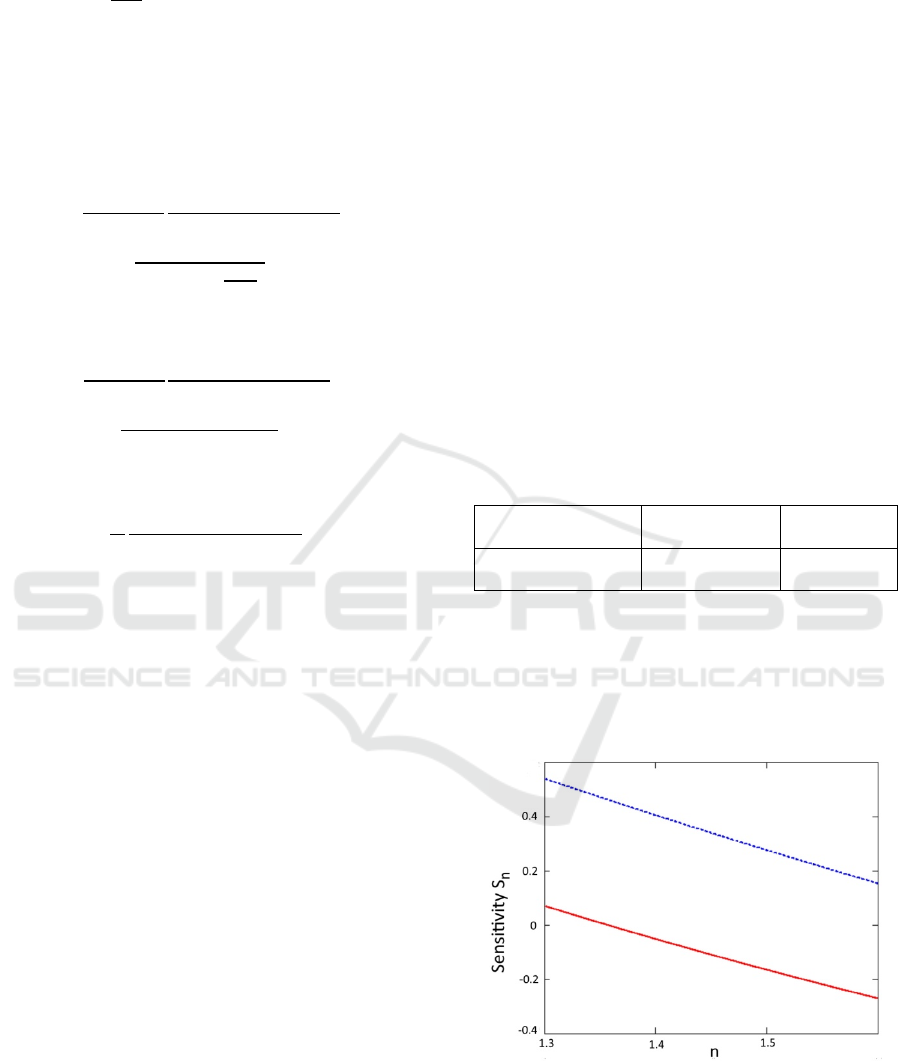
Besides, we have calculated sensitivities of the
correction factor to the change in parameters n and
R
m
, S
n
(see Figure 4), and S
Rm
(see Figure 5),
respectively. For example, the sensitivity to n (S
n
) is
equal to a change (in %) in the correction factor for a
given change (in %) in n: ∆/ =
∆/.
Figure 4: Sensitivity S
n
as a function of the index of
refraction n. Pyoverdine fluorescence (R
x
=0.1, R
m
=0.2) and
porphyrin fluorescence (R
x
=0.1, R
m
=0.4) are depicted by
dotted blue and solid red lines, respectively.
Extraction of Intrinsic Fluorescence in Fluorescence Imaging of Turbid Tissues
127
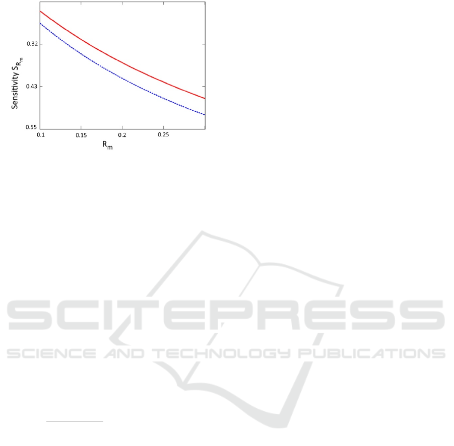
Figure 5: Sensitivity S
Rm
as a function of the reflectance at
emission wavelength R
m
. for different indexes of refraction
1.4 (solid red line) and 1.5 (dotted blue line), respectively.
R
x
was set to 0.1.
4 DISCUSSION
We have obtained explicit equations for the
correction factor if fluorophores are located on the
surface of the tissue (equation (4)) and inside of the
tissue (equation (12)).
We have found that to retrieve intrinsic
fluorescence we need to know diffuse reflectance of
tissue at excitation and emission wavelengths. It can
be embedded into the imaging algorithm: 1) capture
reflectance maps at excitation and emission
wavelengths, 2) calculate the correction factor (per
pixel), 3) apply the correction factor (per pixel) to
retrieve intrinsic fluorescence.
From equations (4) and (12) one can see that the
correction factors have approximately the same
structure (
(
)
(
)
) for fluorophores located
above and below the surface of the tissue. The first
operand (one) corresponds to the nonreflected flow
(external illumination for excitation, and re-emission
in the upper semisphere for fluorescence), while the
second operand corresponds to the reflected flow.
The main difference is an amplification (c>1) of the
optical flux near the border of the tissue with
mismatched boundary conditions.
From equations (4) and (12), one can see that both
the excitation component and emission component
contribute to the correction factor similarly, which is
quite different from Kim’s model (Kim, 2010). We
should note that they assumed a homogeneous
distribution of fluorophores in the tissue, which is not
always a realistic assumption.
From Figures 4 and 5, one can see that the
correction factor is relatively insensitive to errors in
the determination of parameters n and R
m
. For
example, 0.05 error in the determination of the index
of refraction (3.5%) will translate into less than 2%
correction factor error. Likewise, 10% error in
determination of the R
m
will translate into 3-5%
correction factor error. These results can simplify the
correction algorithm by eliminating reflectance
measurements at the excitation wavelength in some
cases. If we consider 400nm range, such as the
sensitivity is quite small (we can use Figure 5 as a
proxy), then even a rough approximation of the
diffuse reflectance (±50% accuracy) will lead to 10-
15% correction factor error. However, for more
precise measurements, capturing R
x
reflectance map
can be helpful.
The coefficient of specular reflection r
s
(
=
( − 1)
/( + 1)
) varies insignificantly with the
wavelength in UVA and visible spectra and stays
within a 2-5% range for biologically relevant indexes
of refraction (n=1.3-1.6). It is reasonable to assume
that the index of refraction stays constant within one
object, so it is not necessary to correct for it within
one image. However, if more accurate quantification
of fluorescence is required, then correction on
specular reflection can be helpful.
In realistic imaging settings, the algorithm
requires certain modifications. An imaging sensor
typically integrates the light over a certain spectral
range. If we take into account that the fluorescence is
typically broadband, then to calculate the correction
coefficient accurately, certain precautions have to be
taken. Ideally, we can measure tissue reflectance at
the whole fluorescence spectra range and then
integrate (4) or (12) over that range. However, in the
first approximation, we can measure tissue
reflectance at fluorescence spectra maximum.
Finally, the proposed model assumes that the
fluorophores form a thin layer within the tissue close
to its surface. This assumption is valid if the thickness
of the layer is significantly smaller than the effective
penetration depth. For example, using optical
parameters for the skin at 400nm
a
= 3.76cm
-1
, and
’
s
= 71.8cm
-1
(Bashkatov, 2011), we can find that
eff
=29.2cm
-1
, Thus, for layers with thickness
l=300m and below and located within 300mm from
the surface (epidermis and upper dermis) that
assumption holds.
In the future, we plan to validate our models in
experiments on absorbing phantoms. In particular, we
plan to use layered phantoms (Saiko, 2018) with an
absorption layer (gelatine and hemoglobins) and a
fluorescence layer (gelatine and quantum dots),
stacked in a sandwich structure.
BIOIMAGING 2020 - 7th International Conference on Bioimaging
128

5 CONCLUSIONS
We have proposed a photon propagation model for
correction of fluorescence on absorption in two
realistic scenarios: when fluorophores are located a)
on the surface of the turbid tissue and b) in a layer
within the turbid tissue. The models require
measurements of diffuse reflection of the tissue at
excitation and emission wavelength and do not
require precise measurement of optical properties
(e.g., coefficient of absorption). The approach can be
implemented using an inexpensive imaging setup and
can be used in any setting.
REFERENCES
Sevick-Muraca E.M., 2012, Translation of Near-Infrared
Fluorescence Imaging Technologies: Emerging
Clinical Applications, An Rev Med, 63: 217-231.
Dartnell L.R, Roberts T.A, Moore G, Ward J.M, Muller J.P.
2013. Fluorescence Characterization of Clinically-
Important Bacteria. PLoS ONE; 8: e75270.
Kjeldstad B, Christensen T, Johnsson A. 1985. Porphyrin
photosensitization of bacteria. Adv. Exp. Med. Biol.
193: 155-159.
Cody Y.S, Gross D.C. 1987. Characterization of pyoverdin
(pss), the fluorescent siderophore produced by
Pseudomonas syringae pv. Syringae. Appl. Environ.
Microbiol. 53: 928-934.
Bradley R. S., Thorniley M. S., 2006, A review of
attenuation correction techniques for tissue
fluorescence. J. Roy. Soc, Interface, 3(6), 1–13.
Liu C. H., Das B. B., Glassman W. L. S., Tang G. C., Yoo
K. M., Zhu H. R, Akins D. L, Lubicz S. S, Cleary J.,
Prudente R, Celmer E, Caron A., and Alfano R. R.,
1992. Raman, fluorescence, and time-resolved light-
scattering as optical diagnostic-techniques to separate
diseased and normal biomedical media, J. Photochem.
Photobiol. B 16~2 187–209.
Anidjar M., Cussenot O., Avrillier S, Ettori D., Villette M.
J., Fiet J., Teillac P., and Le Duc A., 1996. Ultraviolet
laser-induced autofluorescence distinction between
malignant and normal urothelial cells and tissues, JBO.
1, 335–341.
Wu J., Feld M. S., and Rava R. P., 1993. Analytical model
for extracting quantitative fluorescence in turbid media,
Appl. Opt. 32, 3585–3595.
Muller M. G., Georgakoudi I., Zhang Q., Wu J., and Feld
M. S., 2001. Intrinsic fluorescence spectroscopy in
turbid media: disentangling effects of scattering and
absorption, Appl. Opt. 40, 4633–4646.
Pfefer T. J., Schomacker K. T, Ediger M. N, and Nishioka
N. S., 2001. Light propagation in tissue during
fluorescence spectroscopy with single-fiber probes,
IEEE J. Sel. Top. Quantum Electron. 7, 1004–1012.
Kim A., Khurana M., Moriyama Y., and Wilson B. C.,
2010. Quantification of in vivo fluorescence decoupled
from the effects of tissue optical properties using fiber-
optic spectroscopy measurements, JBO. 15(6), 067006.
Valdes P.A., Angelo J.P., Choi H.S, and Gioux S, 2017. qF-
SSOP: real-time optical property corrected
fluorescence imaging, BOE 8, 3597-3605.
Yang B., Tunnell J.B., 2014. Real-time absorption reduced
surface fluorescence imaging, JBO, 19(9), 090505.
Lin W.C, Toms S.A, Jansen E.D, and Mahadevan-Jansen
A, 2001. Interoperative Application of Optical
Spectroscopy in the Presence of Blood, IEEE J. on Sel.
Top. in Quantum Electron, 7(6), 996- 1003.
Zhang Y., Hou H., Zhang Y., Wang Y., Zhu L., Dong M.,
Liu Y., 2018, Tissue intrinsic fluorescence recovering
by an empirical approach based on the PSO algorithm
and its application in type 2 diabetes screening, BOE 9:
1795-1808.
Welch A.J., van Gemert M.J.C., Star W.M., 2011,
Definitions and Overview of Tissue Optics in Optical-
Thermal Response to Laser-Irradiated Tissue, Ed.
Welch AJ, Springer, Dordrecht, NLD, 2
nd
edition.
Star W.M., 2011, Diffuse Theory of Light Transport in
Optical-Thermal Response to Laser-Irradiated Tissue,
Ed. Welch AJ, Springer, Dordrecht, NLD, 2
nd
edition.
Bashkatov A.N., Genina E.A., Tuchin V.V, 2011. Optical
Properties of Skin, Subcutaneous, and Muscle Tissues:
a Review, J. Inn. Opt. Health Sci, 4(1) 9-38.
Saiko G., Zheng X., Betlen A., Douplik A., 2019,
Fabrication and Optical Characterization of Gelatin-
Based Phantoms for Tissue Oximetry, Adv Exp Med
Biol (in press).
Extraction of Intrinsic Fluorescence in Fluorescence Imaging of Turbid Tissues
129
