A Recurrent Neural Network and Differential Equation based

Spatiotemporal Infectious Disease Model with Application to COVID-19

Zhijian Li

, Yunling Zheng

Jack Xin

and Guofa Zhou

Department of Mathematics, University of California, Irvine, U.S.A.

College of Health Science, University of California, Irvine, U.S.A.

Keywords:

COVID-19, Recurrent Neural Network, Discrete Epidemic Model, Spatiotemporal Deep Learning.

Abstract:

The outbreaks of Coronavirus Disease 2019 (COVID-19) have impacted the world signiﬁcantly. Modeling the

trend of infection and real-time forecasting of cases can help decision making and control of the disease spread.

However, data-driven methods such as recurrent neural networks (RNN) can perform poorly due to limited

daily samples in time. In this work, we develop an integrated spatiotemporal model based on the epidemic

differential equations (SIR) and RNN. The former after simpliﬁcation and discretization is a compact model

of temporal infection trend of a region while the latter models the effect of nearest neighboring regions. The

latter captures latent spatial information. We trained and tested our model on COVID-19 data in Italy, and

show that it out-performs existing temporal models (fully connected NN, SIR, ARIMA) in 1-day, 3-day, and

1-week ahead forecasting especially in the regime of limited training data.

1 INTRODUCTION

Susceptible-Infected-Removed (SIR) is a classical

differential equation model of infectious diseases

(Anderson and May, 1992). It divides the total popu-

lation into three compartments and models their evo-

lution by the system of equations

= −β I S

= β I S − γI

= γ I

where β and γ are two positive parameters. SIR is

a simple and efﬁcient model of temporal data for a

given region, see also (Hethcote, 2000) for related

compartment models with social structures.

Yet the infectious disease data are often spatio-

temporal as in the case of COVID-19, see (Italian re-

gion, 2020). A natural question is how to extend SIR

to a space time model of suitable complexity so that it

can be quickly trained from the available public data

sets and applied in real-time forecasts. See (Roosa

et al., 2020) for temporal model real-time forecasts

on cumulative cases of China in Feb 2020.

In this paper, we explore spatial infectious dis-

ease information to model the latent effect due to

the in-ﬂow of the infected people from the geograph-

ical neighbors. The in-ﬂow data is not observed.

To this end, machine learning tools such as regres-

sion and neural network models are more convenient.

Auto-regressive model (AR) and its variants are lin-

ear statistical models to forecast time-series data. The

Long Short Term Memory (LSTM) neural networks,

originally designed for natural language processing

(Hochreiter and Schmidhuber, 1997), have more rep-

resentation power and can be applied to disease time-

series data as well. With spatial structures added, the

graph-structured LSTM models can achieve state-of-

the-art performance on spatiotemporal inﬂuenza data

(Li et al., 2019), crime and trafﬁc data (Wang et al.,

2019; Wang et al., 2018). However, they require a

large enough supply of training data. For COVID-19,

we only have limited daily data since the outbreaks

began in early 2020. Applying space-time LSTM

models (Li et al., 2019; Wang et al., 2018) directly

to COVID-19 turns out to produce poor results.

In view of the limited COVID-19 data, we shall

propose a hybrid SIR-LSTM model where a discrete

time equation for the I-component of SIR model will

be derived and coupled to time dependent features of

neighboring regions through LSTMs.

Li, Z., Zheng, Y., Xin, J. and Zhou, G.

A Recurrent Neural Network and Differential Equation based Spatiotemporal Infectious Disease Model with Application to COVID-19.

DOI: 10.5220/0010130000930103

In Proceedings of the 12th International Joint Conference on Knowledge Discovery, Knowledge Engineering and Knowledge Management (IC3K 2020) - Volume 1: KDIR, pages 93-103

ISBN: 978-989-758-474-9

2 RELATED WORK

In (Yang et al., 2015), the authors designed a vari-

ant of AR, the AutoRegression with Google search

data (ARGO), that utilizes external feature of google

search data to forecast inﬂuenza data from Centers for

Disease Control and Prevention (CDC). Google Cor-

relate is google search trend data that represents the

popularity of an item and its correlated items searched

in Google engine. It is a weekly data that normalized

to range [0, 100]. Based on Google search trend of

inﬂuenza and its correlated items, ARGO is a linear

model that processes historical observations and ex-

ternal features. The prediction of inﬂuenza activity

level at time t, deﬁned as ˆy

, is given by:

ˆy

= u

∑

j=1

t− j

100

∑

i=1

i,t

ARGO is optimized as:

min

α,



− u

−

∑

j=1

t− j

−

100

∑

i=1

i,t



+λ

α||

+ η

β||

+ λ

α||

+ η

β||

where

α = (α

,··· , α

) and

β = (β

,··· , β

100

). The

t− j

’s, 1 ≤ j ≤ 52, are historical observations of pre-

vious 52 weeks and X

i,t

are the google search trend

measures of top 100 terms that are most correlated

to inﬂuenza at time t. Essentially, ARGO is a lin-

ear regression with regularization terms. In (Yang

et al., 2015), ARGO is shown to outperform stan-

dard machine learning models such as LSTM, AR,

and ARIMA.

In (Li et al., 2019), graph structured recurrent

neural network (GSRNN) further improved ARGO

in the forecasting accuracy of CDC inﬂuenza activ-

ity level. The CDC partitions the US into 10 Health

and Human Services (HHS) regions for reporting.

GSRNN treats the 10 regions as a graph with nodes

,··· , v

, and E be the collection of edges (i.e E =

{(v

)|v

are adjacent}). Based on the average

history of activity levels, the 10 HHS regions are di-

vided into two groups, relatively active group, H , and

relatively inactive group, L . There are 3 types of

edges, L − L , H − L , and H − H , and each edge

type has a corresponding RNN to train the edge fea-

tures. There are also two node RNNs for each group

to output the ﬁnal prediction. Given a node (region) v,

suppose v ∈ H . GSRNN generates the edge features

of v at time t, e

v,H

and e

v,L

, by averaging the history

of neighbors of v in the corresponding groups. Next,

the edge features are fed into the corresponding edge

RNNs:

= edgeRNN

H −L

v,L

), h

= edgeRNN

H −H

v,L

)

Then, the outputs of edgeRNNs are fed into the

nodeRNN of group H together with the node feature

of v at time t, denoted as v

, to output the prediction

of the activity level of node v at time t + 1, or y

t+1

= nodeRNN

, f

3 OUR CONTRIBUTION: IeRNN

MODEL

We propose a novel spatiotemporal model integrating

LSTM (Hochreiter and Schmidhuber, 1997) with a

discrete time I-equation derived from SIR differen-

tial equations. The LSTM is utilized to model la-

tent spatial information. The I-equation models the

observed temporal information. Our model, named

IeRNN, differs from (Li et al., 2019; Wang et al.,

2019; Wang et al., 2018) in that a difference equa-

tion with 3 parameters (the I-equation) ﬁts the limited

temporal data. The I-equation is far more compact

than LSTM.

3.1 Derivation of Discrete-time

I-Equation

Based on SIR model, we add an additional feature I

that represents the external infection inﬂuence from

the neighbors of a region. Then the SIR nonlinear

system with I

as external forcing becomes

= −β

S I − β

S I

(1)

= β

S I + β

S I

− γ I (2)

= γI (3)

which conserves the total mass (normalized to 1): S +

I + R = 1. It follows from (3) that

R(t) = R(t

) +

γI dτ

Hence,

S(t) = 1 − I(t) − R(t

) − γ

I dτ

Substituting S(t) into (2) we have:

= (β

I +β

)



1 − I(t) − R(t

) − γ

I(τ)dτ



−γI

Combining forward Euler method and Riemann sum

approximation of the integral, we have a discrete ap-

proximation:

I(t + 1) = (1 − γ)I(t) +



I(t) + β

(t)



KDIR 2020 - 12th International Conference on Knowledge Discovery and Information Retrieval



1 − I(t) − R(t

) − γ

t − t

p + 1

∑

j=0

I(t − j)



As we model I(t) from the beginning of the infection,

we have t

= 0 and R(t

) = 0. We arrive at the follow-

ing discrete time I-equation:

I(t + 1) = (1 − γ)I(t) +



I(t) + β

(t)





1 − I(t) − γ

p + 1

∑

j=0

I(t − j)



(4)

Note that if we let I

(t) = 0, then we have an approx-

imation of I(t) for the original SIR model, which is a

solely temporal model (named I-model):

I(t + 1) = (1 − γ − β)I(t) − βI

(t)

− β γ

p + 1

I(t)

∑

j=0

I(t − j) (5)

In reality, it is hard to know how a population of a

region interacts with populations of neighboring re-

gions. As a result, I

(t) is a latent information that is

difﬁcult to model by a mathematical formula or equa-

tion. In order to retrieve latent spatial information,

we employ recurrent neural networks made of LSTM

cells (Hochreiter and Schmidhuber, 1997), see Fig. 2.

3.2 Generating Edge Feature and

Computing Latent I

Figure 1: Italian Region Map.

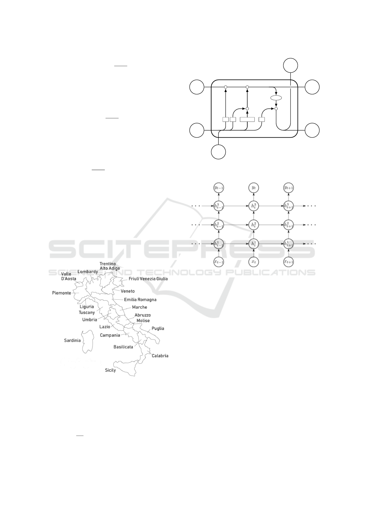
We utilize the spatial information based on the Italy

region map, Fig. 1. In order to learn the latent in-

formation I

of a region v, we ﬁrst generate the edge

feature of v. Let C be the collection of neighbors of v.

Then, the edge feature of v at time t is formulated as:

|C|

∑

i:v

∈C



(t − 1),· ·· , I

(t − p)



σ σ

Tanh

× ×

Tanh

ht−1i

hti

Input

hti

Output

Figure 2: LSTM cell: input x

, output: h

; σ is a sigmoid

function.

Figure 3: Edge RNN consisting of 3 stacked LSTM cells.

where I

(t) is the infection population percentage of

region v

at time t. Then, we feed f

into an Edge

RNN, an RNN with 3 stacked LSTM cells (see Fig.

3), followed by a dense layer for computing I

. The

activation function of the dense layer is hyperbolic

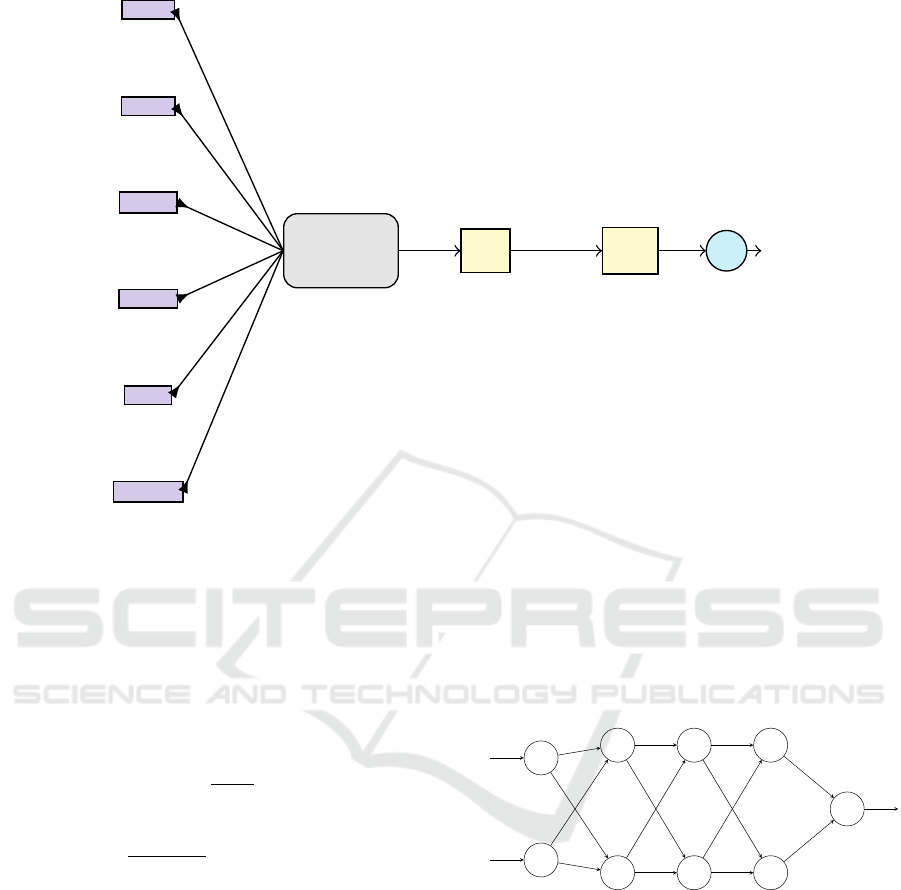
tangent function. Figure 4 illustrates the procedure

of computing I

for Lazio as an illustration. We hence

call our model IeRNN due to its integrated design of

I-equation and edge RNN.

4 EXPERIMENT

To calibrate our model IeRNN, we use the Italy

COVID-19 data (Italian region, 2020) for training and

testing. Although the US has the most infected cases,

the recovered cases are largely missing. On the other

hand, the Italian COVID-19 data is more accurately

reported and better maintained, reﬂecting a nearly

complete duration of the rise and fall of infection.

We collect the data of daily new (current) cases from

2020-02-24 to 2020-06-18 of 20 Italian regions. We

A Recurrent Neural Network and Differential Equation based Spatiotemporal Infectious Disease Model with Application to COVID-19

Tuscany

Umbria

Marche

Abruzzo

Molise

Campania

Edge

Feature

Edge

RNN

Dense

Layer

tanh

Figure 4: Computing I

of Lazio region. Edge RNN is as shown in Fig. 3. Dense layer is fully connected (see Fig. 5).

set p = 3 in (4) based on experimental performance.

As a result, we have the current data for 113 days,

with 81 days to train our model and 32 days to test our

model (or 70%/30% training/testing data split). Our

training loss function is the mean squared error of the

model output and training data:

ˆy(t) = (1 − γ)y(t − 1) +



y(t − 1) + β

(t − 1)





1 − y(t − 1) − γ

p + 1

p+1

∑

j=1

y(t − j)



Loss =

T − p − 1

∑

t=p+1



y(t) − ˆy(t)



Since the training is minimization of the above

loss fucntion over parameters in both I-equation and

RNN, the two components of IeRNN are coupled while

learning from data. We use Adam gradient descent to

learn the weights of LSTM and the dense layer, as

well as I-equation parameters β

, β

, and γ.

To evaluate the performance of our model, we

compare IeRNN, I-model (5), a fully-connected neu-

ral network (fcNN, Fig. 5) with hyperbolic tan-

gent activation function, and auto-regression model

(ARIMA). As the standard setting of ARIMA is 1-

day ahead prediction, we shall only compare with it in

such a very short-term case. Since infectious disease

evolution is intrinsically nonlinear, we shall compare

nonlinear models for 3-day and 1-week ahead fore-

casting. Based on experimental performance, we set

the number of hidden units to be 100, 150, and 100

for the three layers of fcNN respectively.

t−1

t−p

(1)

(2)

(3)

tanh

Input

layer

Hidden

layer

Output

layer

Figure 5: Schematic of fcNN for modeling time series.

4.1 One-day Ahead Forecast

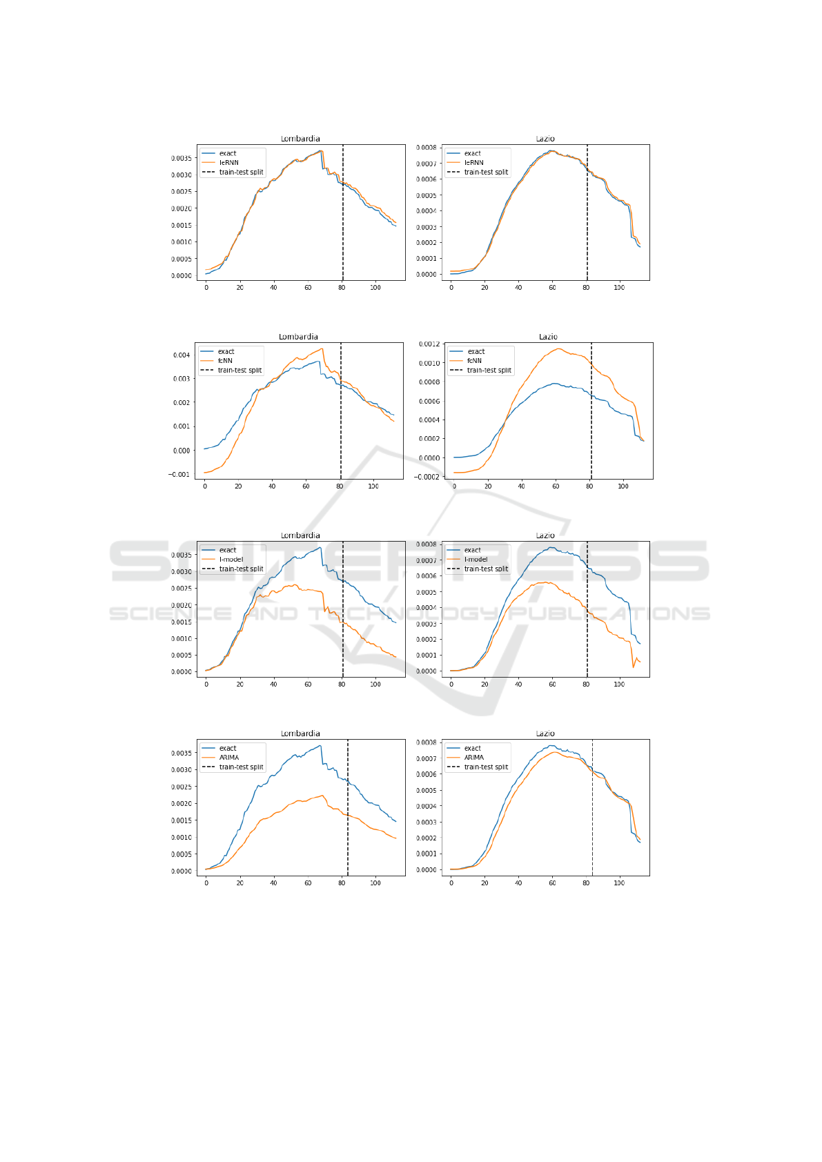
As we see in Fig. 6, fcNN can perform poorly. This

is not a surprise, as both (Li et al., 2019) and (Yang

et al., 2015) relied on hundreds of historical observa-

tions to train their models. The I-model based on only

sequential data in time of one region merely follows

the trend of the true data but cannot provide accurate

predictions. Our IeRNN model, with the help of ad-

ditional spatial information, is able to make accurate

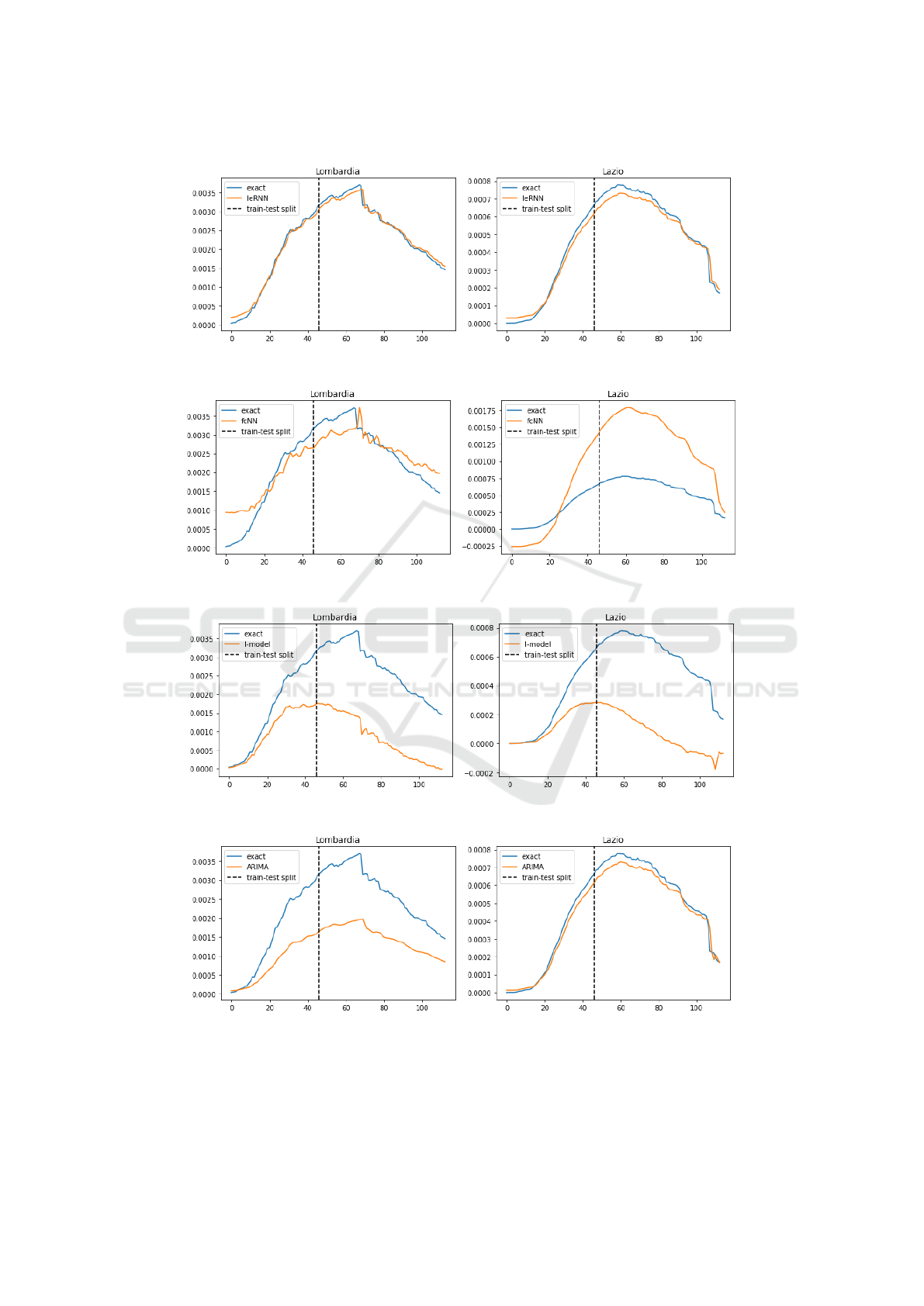
predictions and outperform other models. We also

test the IeRNN with training data reduced to 40% (46

days). IeRNN is still able to track the general trend of

KDIR 2020 - 12th International Conference on Knowledge Discovery and Information Retrieval

(a) Lombardy (b) Lazio

(e) Lombardy (f) Lazio

(g) Lombardy (h) Lazio

Figure 6: Training and 1-day ahead forecast of 4 models (IeRNN, fcNN, I-model, and ARIMA) in 4 rows respectively. The

vertical axis is fraction of newly infected people in the population. The horizontal axis is time in unit of days.

A Recurrent Neural Network and Differential Equation based Spatiotemporal Infectious Disease Model with Application to COVID-19

(a) Lombardy (b) Lazio

(e) Lombardy (f) Lazio

(g) Lombardy (h) Lazio

Figure 7: Training and 1-day ahead forecast of 4 models with reduced (40%) training data. The 4 rows are IeRNN, fcNN,

I-model, and ARIMA respectively. The vertical axis is fraction of newly infected people in the population. The horizontal

axis is time in unit of days.

KDIR 2020 - 12th International Conference on Knowledge Discovery and Information Retrieval

the infected population percentage.

We measure the test accuracy with the Root Mean

Square Error (RMSE) averaged over a few trials in

training. In Tables 1 and 2 on 1-day ahead forecast,

IeRNN achieves the smallest RMSE errors, and I-

model has the largest errors. The compact I-model

with 2 parameters cannot do 1-day ahead prediction

as accurately. ARIMA outperforms I-model and does

better on Emilia-Romagna and Lazio regions than

fcNN. ARIMA, a linear model, has simpler structure

than fcNN whose nonlinearity does not play out in

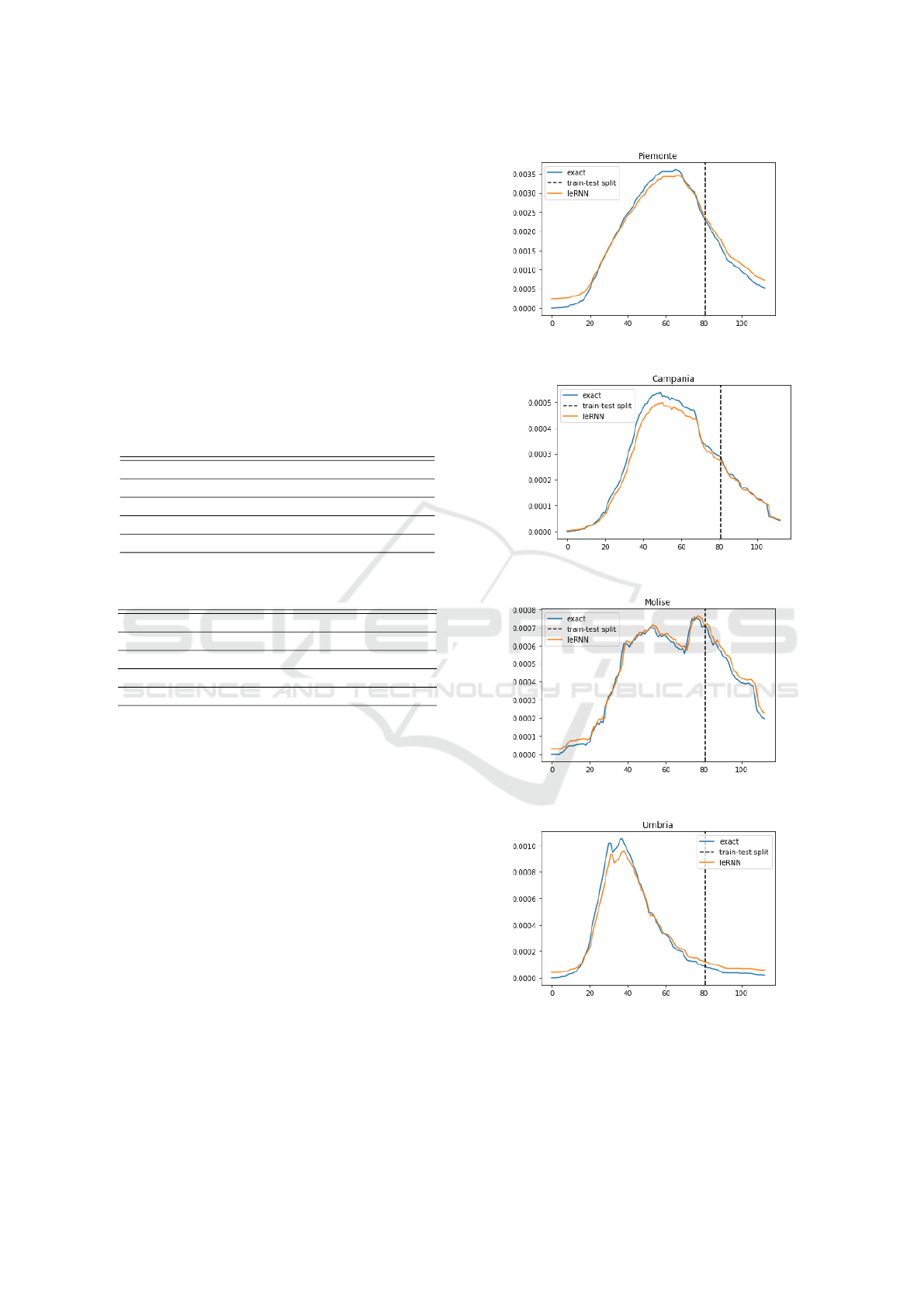
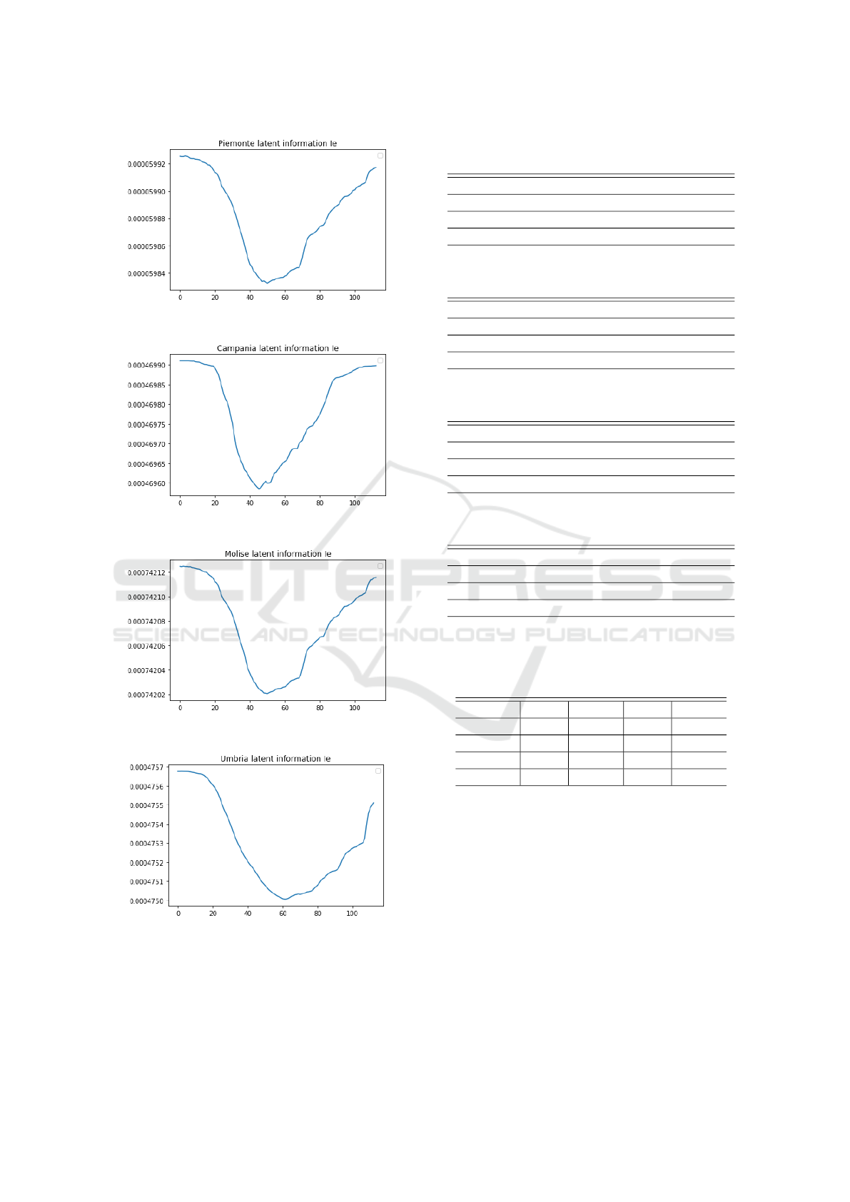
such a short time task. Fig. 8 shows 1-day ahead

forecast of IeRNN model on other regions with the

learned latent external forcing I

in Fig. 9.

Table 1: RMSE test errors in 1-day ahead forecast trained

with 70 % of data. E-R= Emilia-Romagna.

Model Lombardy E-R Lazio

IeRNN 1.027e-04 6.333e-05 3.251e-05

I-model 1.175e-03 3.284e-04 2.439e-04

fcNN 1.580e-04 4.614e-04 2.294e-04

ARIMA 9.789e-04 3.627e-04 4.365e-05

Table 2: RMSE test errors in 1-day ahead forecast trained

with reduced (40 % of) data. E-R= Emilia-Romagna.

Model Lombardy E-R Lazio

IeRNN 9.850e-05 1.778e-04 3.617e-05

I-model 1.871e-03 1.252 e-03 5.443e-04

fcNN 3.364e-04 6.204e-04 8.030e-04

ARIMA 1.277e-03 1.082e-03 4.018e-05

4.2 Multi-day Ahead Forecast

In model training for multi-day ahead forecast, the

training loss function is modiﬁed so that the model

input comes from multiple days in the past. In 7-day

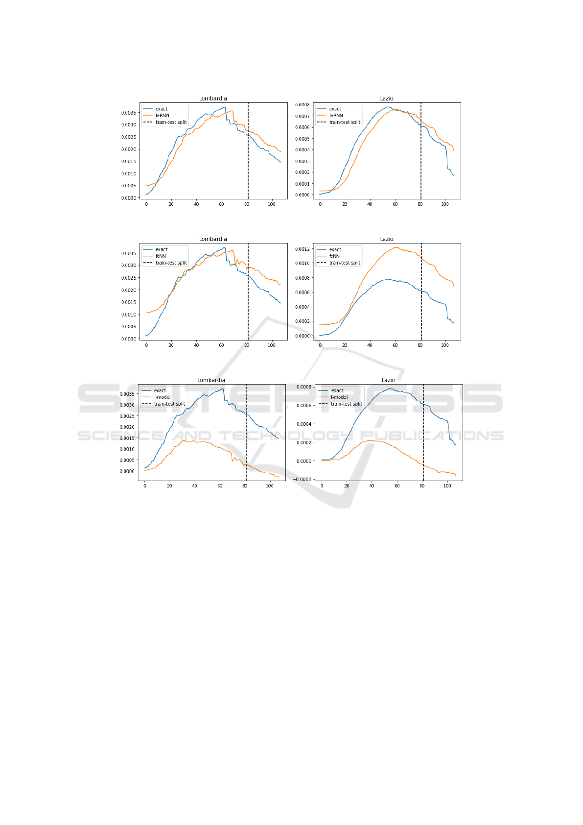
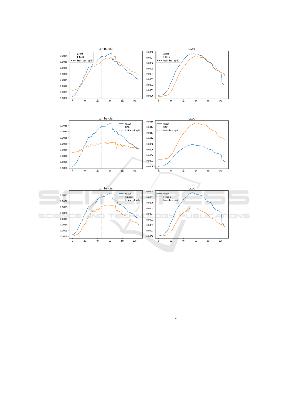
ahead forecast, IeRNN leads the other two nonlinear

models especially in the 40% training data case, by

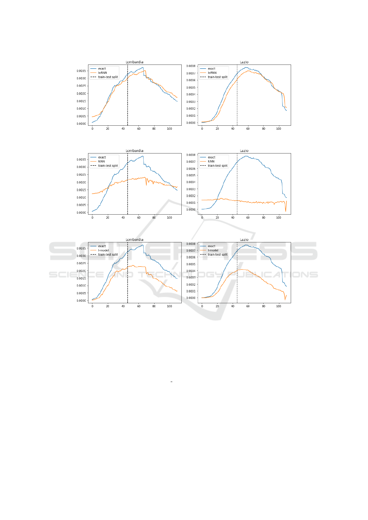
as much as a factor of 7 in Lombardy. In the 3-day

ahead forecast, IeRNN leads fcNN by a factor of 4

in the 40% training data case, as much as a factor of

10 in Lazio. Figs. 10-12 show model comparison in

training and forecast phases for Lombardy and Lazio.

4.3 Model Size and Computing Time

IeRNN (fcNN) has about 16400 (1800) parameters.

The optimized (β

,β

,γ) = (0.685, 0.158, 0.044) in

Lombardy, similarly in other regions. Table 7 lists

average model training and inference times.

(a) Piemonte

(b) Campania

(d) Umbria

Figure 8: IeRNN training and 1-day ahead forecast on four

additional regions.

A Recurrent Neural Network and Differential Equation based Spatiotemporal Infectious Disease Model with Application to COVID-19

(a) Piemonte

(b) Campania

(d) Umbria

Figure 9: Visualization of the latent information I

in Fig. 8

learned by IeRNN.

Table 3: RMSE test errors in 7-day ahead forecast trained

with 70 % of data. E-R= Emilia-Romagna.

Model Lombardy E-R Lazio

IeRNN 3.513e-04 4.423e-04 1.161e-04

I-model 2.004e-03 6.627e-04 5.586e-04

fcNN 6.608e-04 4.804e-04 4.508e-04

Table 4: RMSE test errors in 7-day ahead forecast trained

with reduced (40 % of) data. E-R= Emilia-Romagna.

Model Lombardy E-R Lazio

IeRNN 3.061e-04 4.324e-04 7.754e-05

I-model 2.196e-03 1.167e-03 6.011e-04

fcNN 2.224e-03 6.889e-04 1.851e-04

Table 5: RMSE test errors in 3-day ahead forecast trained

with 70 % of data. E-R= Emilia-Romagna.

Model Lombardy E-R Lazio

IeRNN 2.479e-04 3.668e-04 5.979e-05

I-model 5.609e-04 1.724e-04 1.383e-04

fcNN 8.165e-04 6.757e-04 1.689e-04

Table 6: RMSE test errors in 3-day ahead forecast trained

with reduced (40 % of) data. E-R= Emilia-Romagna.

Model Lombardy E-R Lazio

IeRNN 1.987e-04 3.256e-04 5.297e-05

I-model 1.114e-03 7.337e-04 3.507e-04

fcNN 8.611e-04 1.374e-03 5.290e-04

Table 7: Average model training (tr) and inference (inf)

times in seconds on Macbook Pro with Intel i5 CPU. The

ﬁrst two columns are for 70 % training (tr70) data and the

last two columns are for 40 % training (tr40) data.

Model tr70 inf70 tr40 inf40

IeRNN 0.58s 0.018s 0.51s 0.02s

I-model 0.14s 0.004s 0.11s 0.004s

fcNN 0.09s 0.003s 0.09s 0.003s

ARIMA 0.23s 0.014s 0.19s 0.015s

5 CONCLUSIONS AND FUTURE

WORK

We developed a novel spatiotemporal infectious dis-

ease model consisting of a discrete epidemic equation

for the region of interest and RNNs for interactions

with nearest geographic regions. Our model can be

trained under 1 second. Its inference takes a fraction

of a second, suitable for real-time forecasting and as-

sisting governments in decision making. Our model

out-performs temporal models in one-day and multi-

day ahead forecasts in limited training data regime.

KDIR 2020 - 12th International Conference on Knowledge Discovery and Information Retrieval

100

(a) Lombardy (b) Lazio

(e) Lombardy (f) Lazio

Figure 10: Training and 7-day ahead forecast of 3 models (IeRNN, fcNN, and I-model) in 3 rows respectively. The vertical

axis is fraction of newly infected people in the population. The horizontal axis is time in unit of days.

In future work, we shall study COVID-19 data in

other regions of the world and more sophisticated dif-

ferential equation models such as SEIR

(Anderson and May, 1992; Hethcote, 2000) in our

framework here. It is interesting to derive similar dis-

crete time I-equations. We shall also include a con-

trol mechanism in our model to evaluate various lock-

down and social distancing measures on the evolu-

tion of infections. This will provide a useful tool for

policymakers to assess the impact of their proposed

measures. The ﬁrst step in this direction is to replace

the interaction parameter β

by a parameterized func-

tion of time (Morris et al., 2020) to model government

policies.

Another future direction is to study: 1) trafﬁc data

for understanding interactions and transmissions be-

yond nearest geographic neighbors; 2) social mech-

anism (Albi et al., 2020) to distinguish interactions

among and within different age groups.

ACKNOWLEDGEMENTS

The work was partially supported by NSF grants IIS-

1632935, and DMS-1924548. The authors thank

Prof. Frederic Wan for helpful communications on

disease modeling, and the anonymous reviewers of

KDIR 2020 for their constructive comments.

A Recurrent Neural Network and Differential Equation based Spatiotemporal Infectious Disease Model with Application to COVID-19

101

(a) Lombardy (b) Lazio

(e) Lombardy (f) Lazio

Figure 11: Training and 7-day ahead forecast of 3 models (IeRNN, fcNN, and I-model) with reduced (40%) training data in 3

rows respectively. The vertical axis is fraction of newly infected people in the population. The horizontal axis is time in unit

of days.

REFERENCES

Albi, G., Pareschi, L., and Zanella, M. (2020). Con-

trol with uncertain data of socially structured com-

partmental epidemic models. ArXiv Preprint ArXiv,

2004.13067v1:1–26.

Anderson, R. and May, R. (1992). Infectious Diseases of

Humans: Dynamics and Control. Oxford University

Press, Oxford.

Hethcote, H. (2000). The mathematics of infectious dis-

eases. SIAM Review, 42:599 – 653.

Hochreiter, S. and Schmidhuber, J. (1997). Long short-term

memory. Neural computation, 9(8):1735–1780.

Italian region (accessed March-July, 2020). Italian COVID-

19 Data. https://github.com/Akaza994/COVID-19-

Data/blob/master/covid-19/italy.csv.

Li, Z., Luo, X., Wang, B., Bertozzi, A., and Xin, J. (2019).

A study on graph-structured recurrent neural networks

and sparsiﬁcation with application to epidemic fore-

casting. In World Congress on Global Optimization,

pages 730–739, https://doi.org/10.1007/978–3–030–

21803–4 80. Springer.

Morris, D., Rossine, F., Plotkin, J., and Levin, S. (2020).

Optimal, near-optimal, and robust epidemic control.

ArXiv Preprint ArXiv, 2004.02209v2:1–28.

Roosa, K., Lee, Y., Luo, R., Kirpich, A., Rothenberg, R.,

Hyman, J., Yan, P., and Chowell, G. (2020). Real-

time forecasts of the COVID-19 epidemic in China

KDIR 2020 - 12th International Conference on Knowledge Discovery and Information Retrieval

102

(a) Lombardy (b) Lazio

(e) Lombardy (f) Lazio

Figure 12: Training and 3-day ahead forecast of 3 models (IeRNN, fcNN, and I-model) with reduced (40 %) training data in

3 rows respectively. The vertical axis is fraction of newly infected people in the population. The horizontal axis is time in unit

of days.

from February 5th to February 24th, 2020. Infectious

Disease Modelling, 5:256 – 263.

Wang, B., Luo, X., Zhang, F., Yuan, B., Bertozzi, A., and

Brantingham, J. (2018). Graph-based deep model-

ing and real time forecasting of sparse spatio-temporal

data. MiLeTS ’18, London, UK, DOI: 10.475/123 4;

arXiv preprint arXiv:1804.00684.

Wang, B., Yin, P., Bertozzi, A., Brantingham, J., Osher, S.,

and Xin, J. (2019). Deep learning for real-time crime

forecasting and its ternarization. Chinese Annals of

Mathematics, Series B, 40(6):949–966.

Yang, S., Santillana, M., and Kou, S. C. (2015). Accu-

rate estimation of inﬂuenza epidemics using Google

search data via ARGO. Proceedings of the National

Academy of Sciences, 112(47):14473–14478.

A Recurrent Neural Network and Differential Equation based Spatiotemporal Infectious Disease Model with Application to COVID-19

103