A Neural-Fuzzy System for Predicting the Areal Surface Metrology

Parameters

Ronak Sharma, Mahdi Mahfouf and Olusayo Obajemu

Department of Automatic Controls and Systems Engineering, The University of Shefﬁeld, S1 3JD, Shefﬁeld, U.K.

Keywords:

Model 1, Model 2, ANFIS, Surface Metrology, Sa, Sq, RMSE, RMS, Multi-objective Optimisation.

Abstract:

With the increasing demand for faster manufacturing, Industry 4.0 has now only started to contribute towards

streamlining the manufacturing processes. Despite the availability of high dimensional manufacturing data,

a signiﬁcant amount of time is still spent on testing the end products. Therefore, with a drive to substitute

these inspection processes with a “digital twin”, this paper presents a framework for predicting the optimal

surface metrology parameters such as force and vibration, required to achieve the desired surface roughness

of an end product. Firstly, an Adaptive Neuro-Fuzzy Inference System (ANFIS) was designed to predict

the surface roughness using vibration, force and temperature. A low RMSE of 0.07 was obtained between

the predicted and desired surface roughness. This model was then reverse engineered to predict the optimal

surface conditions (force, vibration and temperature) required to achieve the desired surface roughness. For

this, optimisation was applied to minimise the error between the target and predicted surface roughness. This

framework will help manufacturing industries to discard frequent in-depth product inspection processes in

favour of this “digital twin” due to the possibility of achieving right-ﬁrst-time production.

1 INTRODUCTION

Manufacturing is an ever-developing sector that con-

tinuously strides towards accuracy to ensure the ef-

ﬁcient production of goods. Therefore, industries

are now adopting Multistage Manufacturing Process

(MMP), which involves performing multiple opera-

tions such as forming, machining and assembly in a

series to create the end product(Yang et al., 2010).

To meet the growing demand for customer-centric

products, there has been a rising focus on product

quality. Due to this, a signiﬁcant amount of time is

spent on the testing of end products to ensure that they

meet the stringent customer requirements. Therefore,

the demand to substitute these processes with an alter-

native has given birth to the ﬁeld of surface metrology.

This ﬁeld focuses on the measurement of small-scale

characteristics such as amplitude, spacing and shape

of features of a manufactured product (Yang et al.,

2010). These surface properties are correlated to the

function of a manufactured product and thus play an

important role in predicting its behaviour over time.

Therefore, exploiting surface metrology data can help

discard these physical inspection processes and still

meet the stringent environmental and economic con-

straints to achieve ‘right-ﬁrst-time production’. With

the continuous advancements in data acquisition tech-

nologies, industries are now equipped with cutting

edge sensors for measuring surface properties such

as vibration, force and temperature throughout the

MMP. Therefore, applying Artiﬁcial Intelligence (AI)

techniques can help discover new and not so obvious

patterns, which can then be used to design data-driven

models for simulating these manufacturing processes.

As a result, these models can help compute the op-

timal surface parameters such as force and vibration

required to achieve the desired surface quality such

as roughness thus simplifying the product inspection

process. By providing better insights into the man-

ufacturing processes, these models can further con-

tribute to the diagnostics and prognostics of a product,

thus reducing costs and achieving better customer sat-

isfaction. Considering the above advantages of using

AI for surface metrology, this paper presents a sys-

tems engineering framework, capable of predicting

the optimal surface conditions required for achiev-

ing the desired surface roughness. To achieve this, an

ANFIS model was ﬁrst developed to predict the sur-

face roughness using surface parameters such as vi-

bration. This model was then reverse-engineered and

optimised to predict the optimal surface parameters

required to achieve the desired surface roughness.

286

Sharma, R., Mahfouf, M. and Obajemu, O.

A Neural-Fuzzy System for Predicting the Areal Surface Metrology Parameters.

DOI: 10.5220/0010125602860293

In Proceedings of the 12th International Joint Conference on Computational Intelligence (IJCCI 2020), pages 286-293

ISBN: 978-989-758-475-6

 2020 by SCITEPRESS – Science and Technology Publications, Lda. All rights reser ved

2 LITERATURE REVIEW

2.1 Rise of Surface Metrology

Achieving a good surface ﬁnish ensures that the cus-

tomer desired tribological properties such as high fa-

tigue strength, corrosion resistance and aesthetic ap-

peal are met to a high accuracy(Yang et al., 2017).

However, excessive surface ﬁnishing can lead to in-

creased costs of manufacturing and degraded mechan-

ical properties. As a result, it is important to devise

models that can predict the optimal surface metrol-

ogy parameters required to achieve such properties to

a high degree of accuracy. (Acayaba and de Escalona,

2015) developed an ANN model comprised of two

hidden layers, to predict the surface roughness of

stainless steel in turning. This model achieved an ac-

curacy of 98% thus inspiriing to use an ANN based

technique in this paper for predicting surface rough-

ness. This research also compared the results against

regression models and as expected, ANN performed

better due to a lower Mean Squared Error (MSE). In

another research (Abbas et al., 2018), a multi-layer

perceptron based ANN model was designed to predict

the surface roughness of magnesium alloys used in

aviation products. Using the cutting speed and depth

of cut of the tool as inputs, this model achieved a re-

liable prediction accuracy of 1.35%.

With advancement in AI techniques, an intelligent

framework combining ANFIS and Genetic Algorithm

(GA) was developed to predict the surface roughness

of a thermally drilled hole in galvanised steel (Kumar

and Hynes, 2020). Using the spindle speed and an-

gle of tool as inputs, the ANFIS model predicted the

surface roughness which was then used by GA to min-

imise an objective function. This framework achieved

a correlation of 0.99 and RMSE of 2.4x10

−6

between

the predicted and experiment value.

The above research work shows the advantage of

using AI based frameworks for predicting surface

roughness of manufactured products. Another re-

search showcased the correlation between surface

roughness and surface metrology parameters such as

force and vibration (Rao and Murthy, 2018). Hence,

this paper presents a new system for intelligent man-

ufacturing that combines the above discussed insights

and techniques thus highlighting its novelty. This

framework utilises and learns from surface metrology

data to better predict the surface roughness value of a

manufactured product as a measure of surface quality.

2.2 ANFIS

ANFIS is a feed-forward adaptive neural network

which uses a fuzzy inference system through its struc-

ture.Being a combination of fuzzy logic and neu-

ral network, it provides the advantages of both these

modelling techniques in a single framework i.e. a

powerful interpolator which is transparent and can

deal with uncertainty intrinsically. Such integration is

beneﬁcial because the fuzzy logic manages the impre-

cision and uncertainty while the neural network en-

sures adaptation. The research deﬁned in Section 2.1

shows the popularity of using ANN in surface metrol-

ogy and thus, it was decided to use MATLAB ANFIS

editor (an f isedit) for predicting surface roughness.

Overview: The rest of the paper is organised as

follows. Section 3 describes the experimental set-

up. Section 4 and 5 explain and compare two AN-

FIS models for predicting surface roughness of end

products. Section 6 describes the reverse-engineering

framework that computes the optimal surface param-

eters. Section 7 presents the concluding remarks.

3 EXPERIMENTAL SETUP

A total of seventeen blocks of material steel EN24

were manufactured in the Advanced Manufacturing

Research Centre (AMRC) facility in Shefﬁeld, UK,

where they underwent MMP. These blocks were ﬁrst

heat treated for hardening and then tempered at high

temperatures to produce blocks that possessed simi-

lar mechanical but different surface properties. Here,

the average temperature was measured using ther-

mocouples but only once as a discrete value for ev-

ery block. Then, milling and turning (referred to

as Operation1 and Operation2) were performed on

these blocks. During this, the vibration and force

values were measured using a dynamometer and ac-

celerometer in three axes i.e. X, Y and Z but were

sampled at different rates thus generating differently

sized datasets. A typical 3D surface plot for the sur-

face metrology measurement of a part is shown in

Figure 1. After MMP, a Coordinate Measuring Sys-

tem (CMS) was used to measure surface properties

called Surface Areal Parameters. These parameters

characterise the full 3D surface of a product and are

standardised in the ISO 25178 (Speciﬁcations, 2012).

This contains a list of industry-standard surface areal

parameters. The two popular parameters are Sa and

Sq and have been described in Table 1. A single dis-

crete value of both of these was recorded by the CMS

as a measure of surface roughness for every block.

A Neural-Fuzzy System for Predicting the Areal Surface Metrology Parameters

287

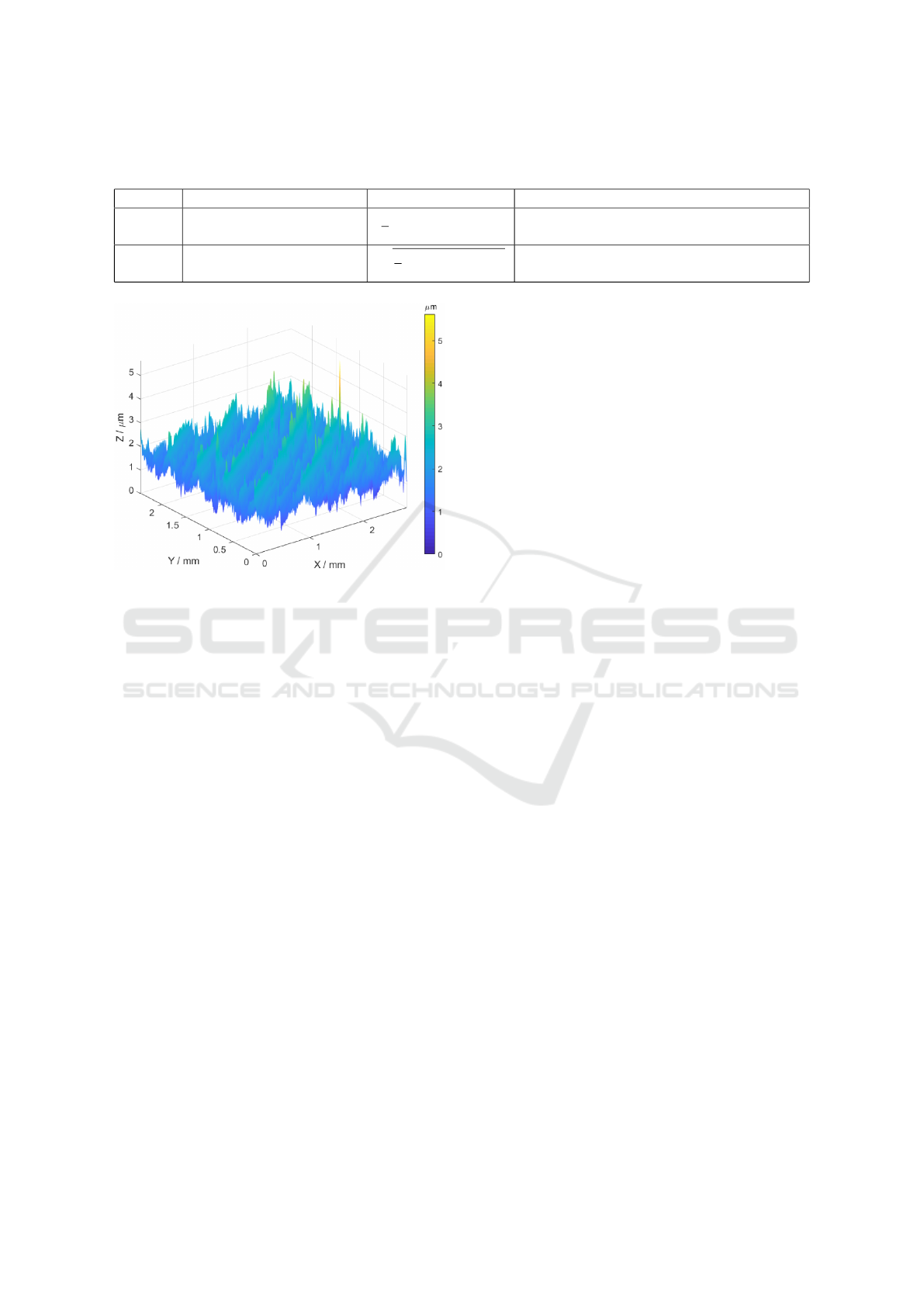
Table 1: Selected areal parameters as deﬁned in the ISO documents. It should be noted that the data is sampled uniformly

along the x and y axes. z(x, y) represents the measured height at location (x, y) (Speciﬁcations, 2012).

Symbol Name Formula Notes

Sa Arithmetic Mean Height

R R

z(x, y))

dxdy

Arithmetic mean of the absolute of the

ordinate values within a deﬁnition area (A).

Sq Root Mean Square Height

R R

(x, y)dxdy

Root mean square value of the ordinate

values within a deﬁnition area (A).

Figure 1: Typical surface metrology measurement of a part.

This is a 3mm x 2.5mm surface patch with a sampling den-

sity of 100 samples per mm(Papananias et al., 2019).

4 MODEL 1: BIN DIVISION

(Rao and Murthy, 2018) showed that vibration mea-

surements were widely used across industries to

predict surface roughness of manufactured products

due to a high correlation between these parameters.

Hence, to produce a simple but reliable model, only

vibration was considered as a useful feature for pre-

dicting the surface roughness. Since Sq had a higher

statistical signiﬁcance than Sa, therefore it was con-

sidered an ideal representation of surface roughness.

4.1 Data Mining

The vibrations during MMP were recorded in three

axes i.e. X, Y and Z and an average correlation of 0.87

was observed between these values. Hence, to ex-

ploit this knowledge, Principal Component Analysis

(PCA) was applied. This reduced the data dimension-

ality by replacing the three axes dataset with a sin-

gle PCA generated dataset thus reducing model com-

plexity without losing any relevant information. Also,

when analysing this PCA’d vibration dataset, it was

identiﬁed that Operation1 data oscillated between -1

and 1, while Operation2 data oscillated between -6

and 6. Therefore, these datasets were then normalised

between 0 and 1 to ensure that the training features

were scaled equally thus reducing the risk of produc-

ing a biased model. The above techniques (PCA and

Normalisation) were applied to the vibration data ob-

tained during both the Operations for all 17 blocks.

4.2 Sample Size Reduction

The above techniques improved the data quality, how-

ever, the I/O dataset was still unequally sized. This

was because the vibration data was a continuous-time

series dataset, however, the Sq data was a discrete

dataset recorded only once for every block. To train a

model, it is important to create a training dataset con-

taining equally sized input and output data. Thus, the

following approach was taken:

• Input Data: The vibration dataset was ﬁrst di-

vided into eight equally sized sub-datasets called

as ‘Bins’. Then, the mean vibration value was cal-

culated for each of these eight ‘Bins’. As a result,

this technique afﬁliated each block with eight vi-

bration values, irrespective of the original dataset

size. This ensured that every block had the same

number of vibration sample values.

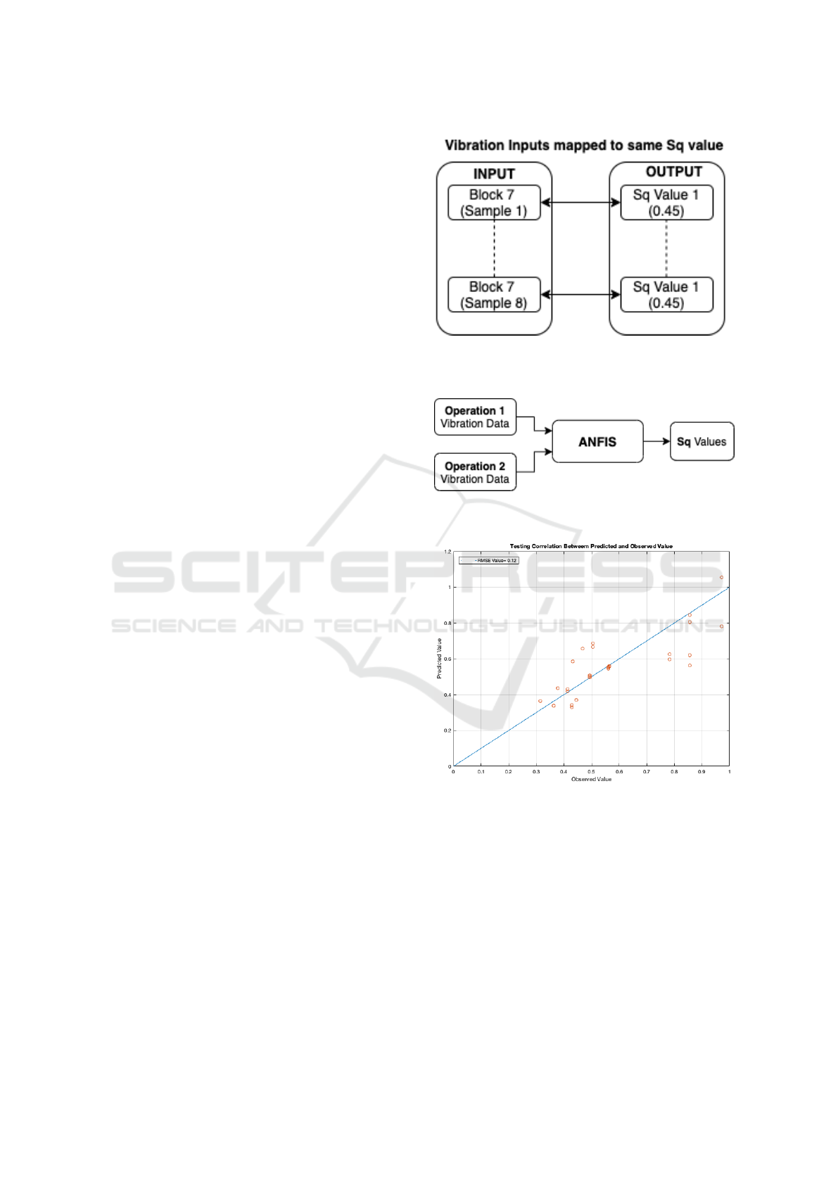
• Output Data: The Sq dataset size was increased

by repeating the same Sq value eight times per

block thus afﬁliating these values to each of eight

mean vibration values as shown in Figure 2.

The above processes were applied to the vibra-

tion dataset obtained for each block during both

Operation1 and Operation2. This resulted in an

equally sized I/O dataset and hence ﬁt for training.

4.3 Overarching Model Architecture

Since all seventeen blocks were identical and under-

went the same Operations, it was decided to combine

the newly processed vibration data of all the seven-

teen blocks obtained from Operation 1 together and

similarly combine the newly processed vibration data

of all blocks obtained from Operation 2 together. This

allowed utilising the vibration data of both Operations

separately for training the model. Figure 3 shows this

model architecture which is a Two Input Single Out-

put ANFIS model. A total of 136 samples were gen-

FCTA 2020 - 12th International Conference on Fuzzy Computation Theory and Applications

288

erated and randomised such that 76% of it were used

for training the model and the rest for testing.

4.4 Further Analysis

Data Filtering: To reduce the effect of outliers, Sav-

itzky Golay ﬁlter was applied to the dataset. How-

ever, this degraded the performance signiﬁcantly as

evidenced by a high RMSE value of 2.34.

Bin Size Adjustments: The performance degraded

with increasing the Bin size (example to 15) possibly

due to overﬁtting. Reducing the Bin Size (example to

4) also led to reduced performance due to underﬁtting.

Hence, Bin size of eight was considered optimal.

4.5 Results and Discussion

The correlation plot in Figure 4 shows that the pre-

dicted Sq values are scattered in the close vicinity

of the correlation line thus evidencing a good perfor-

mance. Correlation of 0.85 and RMSE of 0.12 was

achieved, thus showing the model’s capability for pre-

dicting Sq values to high accuracy. The generalisation

of this model can be evidenced by the training data re-

sponse. A correlation of 0.90 and an RMSE of 0.08

was achieved thus conﬁrming the absence of overﬁt-

ting. Furthermore, a linear regression model and a 2

layer feed-forward ANN were designed and used as

benchmarks to compare the performance. Both these

models obtained a higher RMSE and a lower corre-

lation value thus showing an inferior performance.

Therefore, ANFIS was the preferred technique.

5 MODEL 2: STATISTICAL

FEATURE EXTRACTION

Despite showing a good performance, “Model 1”

posed the following limitations. Firstly, applying

“Bin Division” as explained in Section 4.2 led to a

huge reduction in vibration dataset, thus losing use-

ful information Secondly, the duplication of Sq values

meant providing misleading data to train the model.

Hence, inspired by (Papananias et al., 2019), the fol-

lowing strategy was adopted.

5.1 Data Mining

Based on (Papananias et al., 2019), it was found that

parameters such as force, vibration and temperature

were highly correlated to surface roughness. There-

fore, these features were used for eliciting a new

model i.e. Model 2 for predicting surface roughness

Figure 2: Shows the duplication of Sq values for Block

7, Operation 1. Here, the different vibration values are

mapped to the same Sq value.

Figure 3: Shows an ANFIS model i.e. ‘Model 1’ designed

to predict the Sq values using vibration data.

Figure 4: Testing data shows a near linear relationship b/w

the ‘Model 1’ predicted and observed Sq value.

of end products. Inspired from paper (Papananias

et al., 2019), it was decided to use Sa instead of Sq

as a measure of surface roughness.

Data Set: Vibration and Force, both were continuous

time-series data while temperature and Sa both were

discrete values recorded once for every block. Un-

like Model1, where the focus was to utilise the actual

values of the continuous time-series data, this method

instead focused on utilising the statistical features of

the continuous time-series data as follows.

A Neural-Fuzzy System for Predicting the Areal Surface Metrology Parameters

289

Technique: The Root Mean Square (RMS) and Mean

value of both ‘Force’ and ‘Vibration’ datasets were

calculated for every block. For example, Block 1

had (RMS and Mean) ‘Force’ values and (RMS and

Mean) ‘Vibration’ values afﬁliated to it. This feature

extraction technique was applied to both Operation1

and Operation2 datasets, thus generating eight values

of ‘Force’ and ‘Vibration’ for every block. The tem-

perature was a single value measured only once across

both Operation1 and 2 for every block. Hence, the

ﬁnal training dataset comprised of 17 sample values

due to 17 blocks and each sample was associated with

the above mentioned nine features. Following such a

technique, ensured that the input and output datasets

could now be mapped easily without having to either

reduce the input dataset or duplicate the output values.

Hence, this technique embedded in an ANFIS frame-

work highlights the novelty proposed by this paper.

5.2 Overarching Model Architecture

Figure 5 shows the proposed system architecture. The

nine feature dataset as described above was subjected

to some feature extraction techniques and was then

used as input to an ANFIS model for predicting the

Sa value. The proposed model is a three-input single-

output Sugeno based ANFIS. This architecture over-

came the limitations of ‘Model 1’ as now each block

was linked to nine distinct features, all mapped to a

single Sa value thus avoiding any duplications.

5.3 Feature Extraction

To remove any biases, the sample dataset was ran-

domised. Furthermore, it was identiﬁed that the vi-

bration, force and temperature data were all scaled

differently. Therefore, to ensure equal contribution to

the model design, they all were normalised to a com-

parable scale i.e. between 0 and 1. Having nine input

features but only 17 data samples, such a dataset was

considered unﬁt for model training. Therefore, PCA

was applied to reduce the dimensionality and retain

the useful information of the removed features;

PCA Method: The four vibration values (i.e. RMS

and Mean from both Operation 1 and 2) were ﬁrst col-

lected together and then subjected to PCA thus reduc-

ing the dimension of vibration dataset from four to

one. The same method was then applied to the four

force associated features thus reducing their dimen-

sionality to one. Following this method, the dimen-

sionality of the training dataset was reduced from nine

features at the start to three input features, i.e. PCA’d

Vibration, PCA’d Force and Temperature as shown in

Figure 5. Due to the small sample size (i.e. seven-

teen samples), it was decided to utilise 13 samples for

training i.e. a 76% and 24% split of the data.

Veriﬁcation and Validation

Multiple Runs: The developed ANFIS model was

executed 100 times such that the original dataset was

randomised in each run thus producing a different

RMSE and Correlation value. This was done to ev-

idence the generalisability of the model. Therefore to

evaluate the performance, average RMSE and Corre-

lation values were calculated.

K-Fold Cross Validation: Despite the reduced di-

mensionality, such a low number of data samples

posed the risk of overﬁtting. Hence, 4 Fold Cross-

validation was applied. The performance was eval-

uated by calculating the average Correlation and

RMSE value obtained in each fold. This was used

to evidence the model’s diversity and robustness.

5.4 Results and Discussion

An average correlation and RMSE of 0.87 and 0.09

was obtained on running the model 100 times using

the testing data thus showing acceptable performance.

Figures 6 and 7 show the best predicted and observed

Sa values obtained among the 100 runs using test-

ing and training data. A low RMSE of 0.07 and

0.05 shows the high accuracy of the predictor. Fur-

thermore, the results obtained from the 4-Fold cross-

validation also showed a high correlation and a low

RMSE value for both the training and testing dataset,

thus evidencing model’s generalisability. The 3D sur-

face plots between the input and output, correspond-

ing to this single best run are shown in Figure 8 and

Figure 9.These plots are non-linear and within the

data minimum and maximum ranges thus suggesting

that no obvious extrapolation occurred. Furthermore,

a linear regression model and a 2 layer feed-forward

ANN were designed and used as benchmarks to com-

pare the performance. Both these models produced a

higher RMSE and a lower correlation value than the

ANFIS model thus showing an inferior performance.

Comparison between Model 1 and Model 2

Model2 achieved a lower RMSE and a higher Corre-

lation value. Some other differences were as follows:

• Model1 followed a “Bin Division” approach, util-

ising the actual dataset values thus leading to in-

formation loss. While Model2 utilised the statis-

tical features of the dataset to predict the surface

roughness and thus the preferred choice

FCTA 2020 - 12th International Conference on Fuzzy Computation Theory and Applications

290

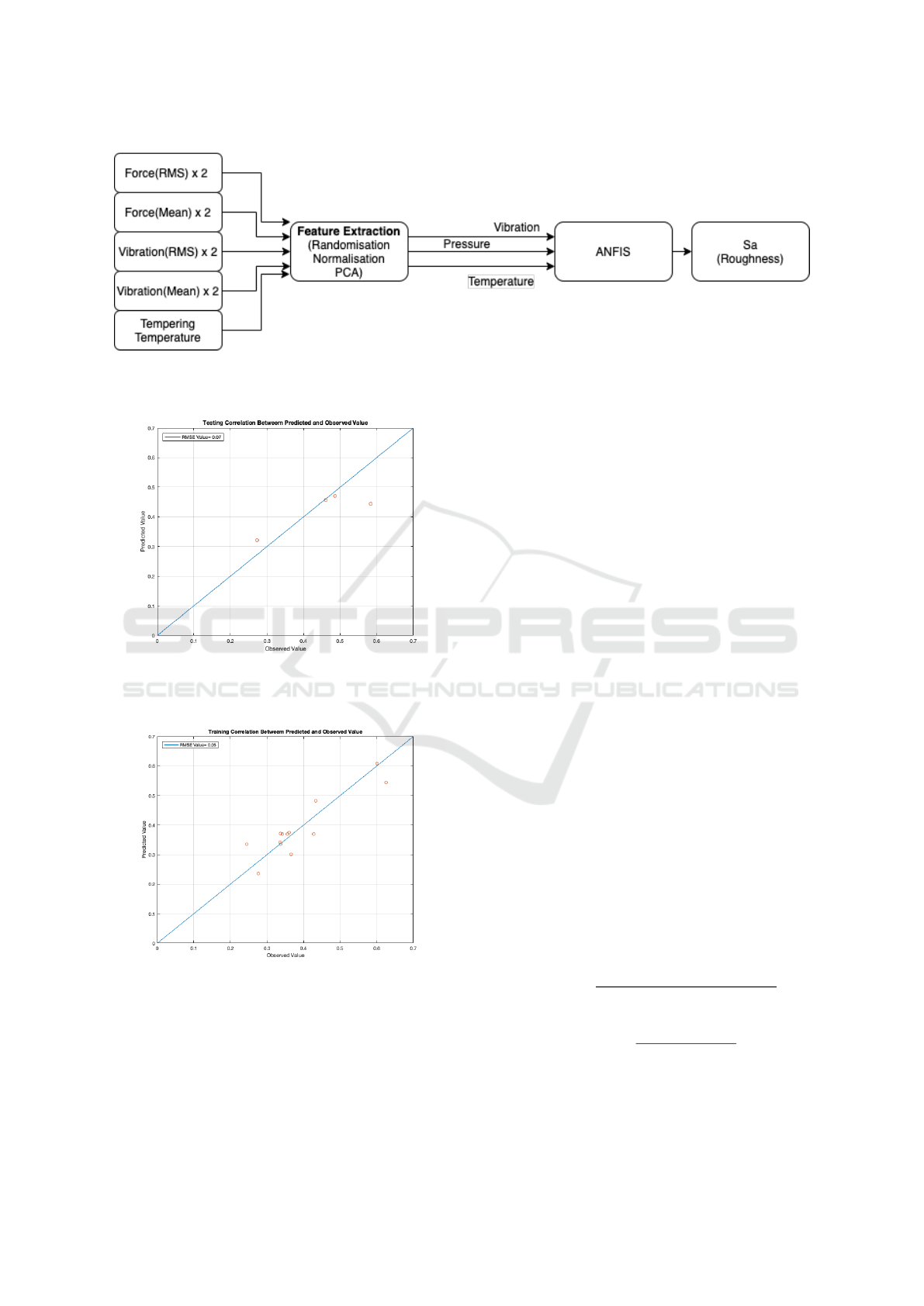
Figure 5: Shows the system architecture of ‘Model 2’.

Figure 6: Testing data shows a linear relationship b/w the

‘Model 2’ predicted and observed Sa value.

Figure 7: Training data shows a linear relationship b/w the

‘Model 2’ predicted and observed Sa value.

• Unlike Model1, Model2 did not require to dupli-

cate the output values i.e. surface roughness val-

ues, thus generating an unbiased training dataset

6 OPTIMISATION FRAMEWORK

6.1 Motivation

The above proposed ‘ Model 2’ was capable of pre-

dicting the surface roughness i.e. Sa value, given

surface metrology parameters as input. However, to

achieve right-ﬁrst-time production, it was required

to design a framework, such that given a target Sa

value as an input, the framework could predict the

optimal surface metrology values required to achieve

that target. Therefore, the following framework

was designed in which the ‘Model 2’ was reverse-

engineered. To achieve this, multi-objective optimi-

sation was applied to minimise the error between the

customer desired and model predicted Sa value until

the error value was below a deﬁned threshold.

6.2 Objective Function

Genetic Algorithm (GA) was used for optimising two

objective functions. The ﬁrst objective was to min-

imise the error between the customer desired and

model predicted Sa value. The second objective was

to minimise the Standard Deviation (SD). Therefore,

multiple predictors were designed which were vari-

ations of ‘Model 2’ . Inspired from (Mason et al.,

2017), these objective functions were also normalised

to minimise the risk of biasness during optimisation.

Mathematically;

Objective 1 =



SaTarget − MeanSaValue(x)

SaTarget



(1)

Objective 2 =



ST DSaValue(x)

SDEstimate



(2)

where, ‘MeanSaValue’ calculated the average of

the Sa value predicted by the multiple models;

‘ST DSaValue’ calculated the SD using the Sa value

A Neural-Fuzzy System for Predicting the Areal Surface Metrology Parameters

291

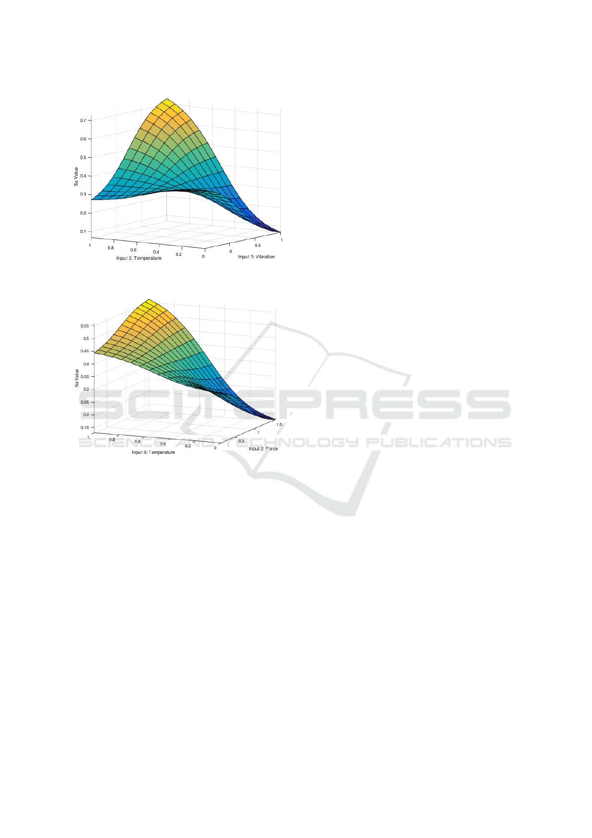
Figure 8: Shows 3D surface plot of Temperature and Vibra-

tion against Sa values.

Figure 9: Shows 3D surface plot of Temperature and Force

against Sa values.

predicted by the multiple models; ‘SDEstimate’ was

set to 1000 (Mason et al., 2017). ‘SaTarget’ was the

customer desired Sa value.

6.3 System Architecture

Figure 10 shows the framework used for reverse-

engineering the proposed ANFIS model. Seven AN-

FIS predictors were designed by varying the Member-

ship Functions(MFs) such as ‘Bell’ and ‘Sigmoid’.

In the ﬁrst iteration of this framework, GA generated

a random set of solution and passed this solution set

to the seven ANIFS models as an input. This solution

set represented the nine features as described earlier

in Figure 5. In each iteration, the seven variations of

‘Model 2’ used the GA produced solution set to pre-

dict seven Sa values. These seven values were then

used to calculate the mean Sa value and SD which

were then passed to the optimiser(GA). Using these

values, the optimiser produced a new set of solutions,

with an aim to minimise the error objective.

6.4 Implementation

Method 1: MATLAB function called gamultiob j

was used for multi-objective optimisation. The objec-

tives were speciﬁed in two separate equations (Sec-

tion 6.2) but were optimised simultaneously. This

produced Pareto solutions. Figure 11 shows that the

solutions for Sa of 0.37, minimised the objectives to

achieve a low MSE in the range of 0.4 and 10

−8

Method 2: Inspired from paper (Mason et al., 2017),

the two objective functions were combined to form

a single function and each objective was assigned a

weight vector to quantify their priorities. This pro-

vided more control over optimisation by allowing

to generate solutions of interest directly rather than

Pareto solutions;

Objective = w1 ∗ (Ob jective1) + w2 ∗ (Ob jective2)

(3)

where w1 and w2 were the weights assigned to each

objective and were varied between 0 and 1. This was

because the objectives themselves were normalised

between this range of values.

6.5 Results and Discussion

Both ‘Method 1’ and ‘Method 2’, produced very sim-

ilar results. However, there was a qualitative differ-

ence between the two methods.

Method 1: This is beneﬁcial for solving generic prob-

lems, where the decision-maker (usually analysts) are

unable to determine the priority order of the different

objectives as they are debatable and not stringent.

Method 2: This is beneﬁcial for solving problems

where analysts can prioritise objectives according to

their goal by manipulating weights of each objective

For the proposed surface metrology problem,

‘Method 1’ was preferred as it provides analysts with

the ﬂexibility to choose the optimal solution that

meets their goals from a range of Pareto solutions.

7 CONCLUSIONS

The increasing demand for customer-centric products

is difﬁcult to meet when a signiﬁcant amount of

time is still spent on the testing of end products.

Therefore, with a drive to substitute these inspection

processes with a ‘digital twin’, this paper presented

FCTA 2020 - 12th International Conference on Fuzzy Computation Theory and Applications

292

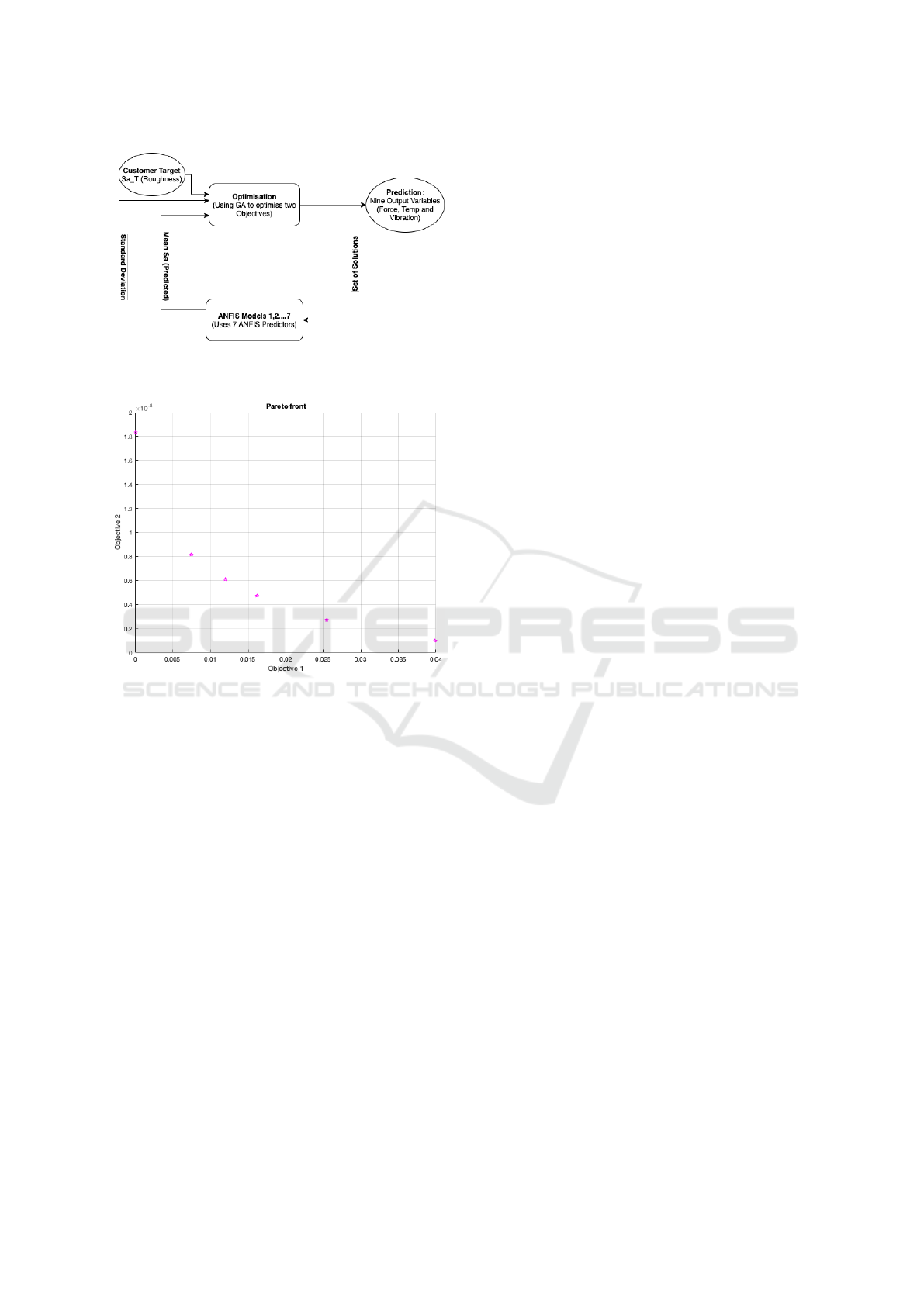
Figure 10: Shows the reverse-engineered framework devel-

oped for achieving right ﬁrst time production.

Figure 11: Pareto-Optimal solutions obtained using

‘Method 1’ where target Sa value was set to 0.37.

an intelligent framework to predict the optimal

surface metrology parameters required for achieving

the desired surface roughness of an end product. This

was a two-stage process:

Stage 1: A 3 I/O ANFIS model was designed

to predict the surface roughness of an end product

using surface parameters such as vibration and force.

Using statistical features of these parameters in an

ANFIS model showcases the novelty.

Stage 2: ‘Model 2’ was then reverse-engineered to

compute the optimal surface metrology values such

as force and vibration required to achieve the desired

surface roughness value. An optimisation framework

was developed where GA was applied to minimise

the error between the predicted and target roughness.

Limitation and Future Work: ‘Model 2’ was

derived using the data collected from seventeen

experiments only. Such a low sample size does not

guarantee a reliable model and hence, more data shall

be collected for robust validation. Due to limited data,

the model was only tested within a limited range of

target values. Hence, the model shall be tested with a

wide range of target values. Another case study shall

also be conducted to establish emphatically that the

proposed framework for digital twin establishment

is generic to a wide range of manufacturing systems.

Finally, other modelling techniques such as SVM and

Deep Learning will be explored as ANFIS can be

restrictive in problem-speciﬁc parameter tuning.

To summarise, developing such a framework for pre-

dicting the surface roughness, will help manufactur-

ing industries to discard the in-depth product inspec-

tion process thus saving on processing time and costs.

REFERENCES

Abbas, A. T., Pimenov, D. Y., Erdakov, I. N., Taha, M. A.,

Soliman, M. S., and El Rayes, M. M. (2018). Ann sur-

face roughness optimization of az61 magnesium alloy

ﬁnish turning: Minimum machining times at prime

machining costs. Materials, 11(5):808.

Acayaba, G. M. A. and de Escalona, P. M. (2015). Pre-

diction of surface roughness in low speed turning of

aisi316 austenitic stainless steel. CIRP Journal of

Manufacturing Science and Technology, 11:62–67.

Kumar, R. and Hynes, N. R. J. (2020). Prediction and

optimization of surface roughness in thermal drilling

using integrated anﬁs and ga approach. Engineer-

ing Science and Technology, an International Journal,

23(1):30–41.

Mason, K., Duggan, J., and Howley, E. (2017). Multi-

objective dynamic economic emission dispatch using

particle swarm optimisation variants. Neurocomput-

ing, 270:188–197.

Papananias, M., McLeay, T. E., Mahfouf, M., and Kadirka-

manathan, V. (2019). A bayesian framework to es-

timate part quality and associated uncertainties in

multistage manufacturing. Computers in Industry,

105:35–47.

Rao, K. V. and Murthy, P. (2018). Modeling and optimiza-

tion of tool vibration and surface roughness in boring

of steel using rsm, ann and svm. Journal of intelligent

manufacturing, 29(7):1533–1543.

Speciﬁcations, G. P. (2012). Surface texture: Areal—part

2: Terms, deﬁnitions and surface texture parameters.

International Standard ISO, pages 25178–2.

Yang, A., Han, Y., Pan, Y., Xing, H., and Li, J. (2017). Op-

timum surface roughness prediction for titanium alloy

by adopting response surface methodology. Results in

Physics, 7:1046–1050.

Yang, Z., Gu, X., Liang, X., and Ling, L. (2010). Ge-

netic algorithm-least squares support vector regres-

sion based predicting and optimizing model on carbon

ﬁber composite integrated conductivity. Materials &

Design, 31(3):1042–1049.

A Neural-Fuzzy System for Predicting the Areal Surface Metrology Parameters

293