Classification and Calibration Techniques in Predictive Maintenance: A
Comparison between GMM and a Custom One-Class Classifier
Enrico de Santis
a
, Antonino Capillo
b
, Fabio Massimo Frattale Mascioli
c
and Antonello Rizzi
d
Department of Information Engineering, Electronics and Telecommunications,
University of Rome “La Sapienza”, Rome, Italy
Keywords:
Predictive Maintenance, Machine Learning, Gaussian Mixture Models, Faults Modeling, One-Class Classifi-
cation.
Abstract:
Modeling and predicting failures in the field of predictive maintenance is a challenging task. An impor-
tant issue of an intelligent predictive maintenance system, exploited also for Condition Based Maintenance
applications, is the failure probability estimation that can be found uncalibrated for most standard and cus-
tom classifiers grounded on Machine learning. In this paper are compared two classification techniques on
a data set of faults collected in the real-world power grid that feeds the city of Rome, one based on a hy-
brid evolutionary-clustering technique, the other based on the well-known Gaussian Mixture Models setting.
While the former adopts directly a custom-based weighted dissimilarity measure for facing unstructured and
heterogeneous data, the latter needs a specific embedding technique step performed before the training proce-
dure. Results show that both approaches reach good results with a different way of synthesizing a model of
faults and with different structural complexities. Furthermore, besides the classification results, it is offered a
comparison of the calibration status of the estimated probabilities of both classifiers, which can be a bottleneck
for further applications and needs to be measured carefully.
1 INTRODUCTION
Low-cost smart sensors and cloud technologies,
boosted with powerful and efficient communication
networks, enable new tool-boxes, grounded on AI, to
face challenges in predictive maintenance programs,
specifically in modern power grids (Smart Grids). In
fact, leveraging AI models to identify the abnormal
behavior in Medium Voltage (MV) feeders (i.e. faults
and outages) turns equipment sensor data into mean-
ingful, actionable insights for proactive asset main-
tenance, preventing downtime or accidents, meeting
present-day time-to-market requirements. The choice
of the specific predictive model is not straightforward,
especially in real-world applications where they are
adopted in production environments. One of the chal-
lenges is the synthesis of a low structural complex-
ity model able to act as a gray-box - enabling knowl-
edge discovery tasks - useful even as a building block
a
https://orcid.org/0000-0003-4915-0723
b
https://orcid.org/0000-0002-6360-7737
c
https://orcid.org/0000-0002-3748-5019
d
https://orcid.org/0000-0001-8244-0015
for more complex programs within business strategic
plans, such as estimating the impact of environmen-
tal conditions on power grid devices. The measure
of the impact together with the probability of failure
can drive risk analysis programs on the entire power
grid, where technicalities turn into long-term huge
investments programs, hence in decisions taken by
high-level managers. Thus, from the output point of
view, the ML system should provide an interpretable
model with not only a Boolean decision over an event
but even with a calibrated probability (Martino et al.,
2019) of occurrence, because the latter quantity plays
a decisive role in the downstream decision-making
process. As an example, the classifiers proposed in
this study will be adopted for measuring the failure
rate derived from the probability of fault. This infor-
mation will be part of a long-term real-world Con-
dition Based Maintenance program. From the input
side, a real-world application, such as a data-driven
predictive maintenance task in Smart Grids (De Santis
et al., 2013), is likely to deal with heavily structured
patterns (Zhang et al., 2018) requiring many efforts in
feature engineering. Specifically, it consists of build-
ing a set of features and a suitable kernel, where stan-
de Santis, E., Capillo, A., Mascioli, F. and Rizzi, A.
Classification and Calibration Techniques in Predictive Maintenance: A Comparison between GMM and a Custom One-Class Classifier.
DOI: 10.5220/0010109905030511
In Proceedings of the 12th International Joint Conference on Computational Intelligence (IJCCI 2020), pages 503-511
ISBN: 978-989-758-475-6
Copyright
c
 2020 by SCITEPRESS – Science and Technology Publications, Lda. All rights reserved
503

dard ML algorithms – designed to be fed by n-tuples
of real-valued numbers – can safely operate.
The current study was born within the “Smart
Grids intelligence project” (ACEA, 2014; Possemato
et al., 2016; Storti et al., 2015), with the aim of equip-
ping the power grid that feeds the entire city of Rome
– managed by the ACEA (Azienda Comunale Ener-
gia e Ambiente) company – with a poly-functional
Decision Support System, able to recognize in real-
time power failures estimating the probability of fault
depending on environmental conditions and data re-
lated to the power grid devices. Specifically, the
paper offers a multi-level comparison between two
different approaches to classification of faults – the
evolutionary based One-Class classification system
(OCC system) (De Santis et al., 2015; De Santis et al.,
2018b) along with several improvements and the well
known Gaussian Mixture models (GMMs) – starting
from a complex representation of the power grid sta-
tus involving different type of real-world data, such
as time data, weather data, power grid structural data,
load data and unevenly spaced time-series data re-
lated to micro-interruption occurring due to, for ex-
ample, partial discharges. The two levels of compari-
son grounds on the specific feature engineering tech-
niques suited to feed the two different classification
algorithms (input side) and the quality of the output
obtained in terms of classification performances and
calibration of probabilities (output side). In fact, the
modeling and prediction of faults in power grids is a
wide research area (Zhang et al., 2018) where fail-
ure causes are debated (Guikema et al., 2006; Cai
and Chow, 2009) and modeled within the ML setting
(Wang and Zhao, 2009) even in extreme environmen-
tal conditions (Liu et al., 2005).
The current study investigates an embedding
technique for representing complex structured data
(within the family of metric recovery techniques)
allowing the adoption of a standard GMM, beside
an evolutionary classification technique (the already-
cited OCC System) in charge of learning a suit-
able metric for a custom based dissimilarity measure,
where the predictive model is grounded on a cluster-
ing technique, offering the possibility of synthesizing
a gray-box interpretable model. Within this setting, as
a novelty, the output soft decision – the score values of
the classifiers – are evaluated for assessing the usabil-
ity as calibrated probabilities associated to a power
grid status.
The following paper is organized as follows. In
Sec. 2 is provided a description of the data set and the
problem setting within the field of predictive main-
tenance and fault recognition with a description on
how to measure the calibration of output probabili-
ties. Sec. 3 offers a synthetic survey on classifica-
tions techniques, specifically the GMM family and
the OCC System. The experimental setting and the
results are discussed in 4, while conclusion are drawn
in Sec. 5.
2 THE REAL-WORLD DATA SET
The power grid managed by ACEA consists of a se-
ries of MV lines equipped with smart sensors collect-
ing faults data for storing and processing tasks. We
refer to a fault as the failure of the electrical insu-
lation (e.g., cables insulation) that compromises the
correct functioning of the grid. Therefore, what we
call Localized Fault (LF) is actually a fault in which
a physical element of the grid is permanently dam-
aged causing long outages. The available real-world
data set consists in data patterns describing the power
grid states that are classified into standard functioning
states (SFSs) and LFs, that is, to each pattern ζ it is as-
sociated a label y(ζ) : y =
{
LF,SFS
}
. These data pat-
terns have been organized together with ACEA field-
experts and are structured in several features. Basi-
cally a power grid state is composed of two main com-
ponents or group of features, that is one to constitutive
parameters of power grid devices and a second group
related to external causes, intended as “forces”, with a
fast-changing dynamic, that influence the power grid
state. The former are, for example, the cable sec-
tion, the constituent material, etc., while the latter are
the weather and the load condition (De Santis et al.,
2017b; Bianchi et al., 2015). A detailed description
of the selected features can be found in (De Santis
et al., 2015). The features belong to different data
types: categorical (nominal), quantitative (i.e., data
belonging to a normed space) and times series (TSs).
The last one describes the sequence of short outages
that are automatically registered by the protection sys-
tems (known as “Petersen” alarm system) as soon as
they occur. Hence, LFs on MV feeders are character-
ized by heterogeneous data, including weather con-
ditions, spatio-temporal data (i.e. longitude-latitude
pairs and time), physical data related to the state of the
power grid and its electric equipment (e.g., measured
currents and voltages). Thereby, the starting patterns
space is structured and non-metric and, as will be ex-
plained in detail, a suitable embedding needs to be
adopted to deal with ML algorithms designed to work
with real-valued tuples. The data set was validated
by cleaning it from human errors and by completing
in an appropriate way missing data, as explained in
(De Santis et al., 2015; De Santis et al., 2017a).
CI4EMS 2020 - Special Session on Computational Intelligence for Energy Management and Storage
504

3 THE CLASSIFICATION
PROCEDURE
The classification task consists of learning a model M
of a specific oriented process P . This means synthe-
sizing a classifier – a predictive model – where the un-
derlying free parameters are learned feeding a set of
h
x,y
i
pairs to a training algorithm. In other words, the
training process allows learning a decision function f
that, given an input x, returns a predicted class label
ˆy, that is ˆy = f (x,Θ
Θ
Θ), where Θ
Θ
Θ is a set of free param-
eters of the model M . Finally, M = M (
h
x,y
i
n
i=1
,Θ
Θ
Θ),
that is, an instance of the model, in general, will de-
pend on the training pairs
h
x,y
i
n
i=1
and the set of free
parameters Θ
Θ
Θ = [θ
θ
θ,Φ
Φ
Φ], where θ
θ
θ are the learning pa-
rameters (model parameters) and Φ
Φ
Φ is a set of hyper-
parameters, which define the structural complexity of
the model. The latter need a suitable search proce-
dure to be set. If the model is learned over only one
class – namely the target class, because the others are
not available for some reason – we have a One-class
classification problem (Khan and Madden, 2010).
Furthermore, it is possible to distinguish the hard
classification task, where the classifier outputs the la-
bel ˆy, and the soft classification one, where it outputs
a score value – i.e. a real-valued number s – provid-
ing roughly the likeliness that a data pattern belongs
to a suitable class. Probabilistic classifiers returns the
posterior probability P(Y |X) of an output ˆy given an
input x. P will depend even on some model param-
eters Θ
Θ
Θ, not highlighted in the expression above. In
general, the hard decision on a class label can be ob-
tained letting:
ˆy = argmax
y
P(Y = y|X), (1)
that is, for a given input pattern x ∈ X, the decision
rule assigns the output label y ∈ Y to the one corre-
sponding to the maximum posterior probability.
Albeit not all classifiers are probabilistic classi-
fiers, some classifiers such as Support Vector Machine
(SVM) (Cortes and Vapnik, 1995) or Na
¨
ıve Bayes
may return a score s(x) which roughly states the “con-
fidence” in the prediction of a given data pattern x. A
typical decalibrated classifier produces a model that
predicts examples of one or more classes in a pro-
portion which does not fit the original one, i.e., the
original class distribution. In the binary case it can be
expressed as a mismatch between the expected value
of the proportion of classes and the actual one (Bella
et al., 2010). Intuitively, calibration means that when-
ever a forecaster assigns a probability of 0.8 to an
event, that event should occur about 80% of the time
(Kuleshov et al., 2018). A plain methodology adopted
to explore the calibration of a classifier is the Relia-
bility diagram (Murphy and Winkler, 1977) where on
the x-axis are reported the scores (or probability for a
probabilistic classifier), whereas on the y-axis are re-
ported empirical probabilities P(y|s(x) = s), namely
the ratio between the number of patterns in class y
with score s and the total number of patterns with
score s. If the classifier is well-calibrated, then all
points lie on the bisector straight line of the first and
third quadrant, meaning that the scores are equal to
the empirical probabilities. Due to the real-valued
nature of the scores and the fact that it is quite im-
possible to quantify the number of data points shar-
ing the same score, a binning procedure is adopted.
Moreover, in literature can be found a series of cali-
bration techniques, some of which allow estimating a
calibration function (adopting a supervised learning
framework) making scores similar to the empirical
probabilities. More details can be found in (Martino
et al., 2019; Kuleshov et al., 2018). Hence, a well-
suited set of probabilities related to the classification
task of data patterns requires either a well-calibrated
classifier or some additional downstream processing.
To quantify the goodness of the calibration, i.e. how
the probability estimates are far from the empirical
probabilities, two methods have been proposed in lit-
erature: the Brier score (Brier, 1950; DeGroot and
Fienberg, 1983) and the Log-Loss score. Given a se-
ries of N known events and the respective probability
estimates, the Brier score is the mean squared error
between the outcome o (1 if the event has been ver-
ified and 0 otherwise) and the probability p ∈ [0,1]
assigned to such event. In the context of binary clas-
sification, the Brier score BS is defined as
BS =
1
N
∑
N
i=1
(T (y
i
= 1|x
i
) −P(y
i
= 1|x
i
))
2
(2)
where T ( ˆy
i
= 1|x
i
) = 1 if ˆy
i
= 1 and T ( ˆy
i
= 1|x
i
) = 0
otherwise and P( ˆy
i
= 1|x
i
) is the estimated probability
for pattern x
i
to belong to class 1. Likewise the MSE,
the lower the BS value, the better.
The Log-Loss for binary classification is defined
as follows:
LL = −
1
N
∑
N
i=1
[y
i
logp
i
+ (1 −y
i
)log(1 − p
i
)] (3)
and, as per the Brier score, the lower, the better. The
Log-Loss index matches the estimated probability
with the class label with logarithmic penalty. Hence,
for small deviations between ˆy
i
and p
i
the penalty is
low, whereas for large deviations the penalty is high.
In standard ML problems the input to the learn-
ing algorithm is often a real-valued data pattern of
some dimension, while in real-world applications it
is likely disposing of structured data pattern, where
Classification and Calibration Techniques in Predictive Maintenance: A Comparison between GMM and a Custom One-Class Classifier
505

not all attributes lie in a normed space. For exam-
ple, some of that can be graphs, time series, categori-
cal variables, etc. At the same time, some classifiers,
such as SVM or the herein adopted OCC System, are
grounded on a custom-based kernel, in turn, designed
on a custom-based dissimilarity measure able to face
each structured pattern through a suitably designed
sub-dissimilarity measure. In other words, indicating
with ζ
i
= [o
i1
,o
i2
,..., o
iR
] the i-th structured data pat-
tern composed by R structured objects o, a custom-
based dissimilarity measure between ζ
i
and ζ
j
can be
formally expressed as:
d(ζ
i
,ζ
j
;w) = f
d
( f
sub
r
(o
ir
,o
jr
);w) r = 1, 2,...R, (4)
where f
sub
t
(·) is a sub-dissimilarity tailed to the spe-
cific data type (underlying the r-th structured at-
tribute o
r
), f
d
is a compositional relation, with suit-
able properties, that applies on sub-dissimilarities and
can depend on a set of weights parameters w. If
the latter are subject to learning, the problem of the
dissimilarity definition is framed in a metric learn-
ing framework (Bellet et al., 2013) and weights can
help to interpret models, driving knowledge discov-
ery tasks. As stated, some ML algorithms can face
directly with custom-based kernels while others (e.g.
GMM), where working with structured data domains,
need some embedding procedure, hence a methodol-
ogy that allows embedding structured data patterns in
a well-suited algebraic space, such as the Euclidean
space (De Santis et al., 2018a). This procedure
can start from the dissimilarity values, computed by
means of expression (4), collected in a dissimilarity
matrix D ∈ R
n×n
, where D
i j
= d(ζ
i
,ζ
j
;w). Among
the main embedding techniques, it is worth to cite the
possibility of adopting directly the dissimilarity ma-
trix as a data matrix (hence, the rows as real-valued
data patterns in R
n
), eventually reducing the number
of dimensions with some heuristics, such as cluster-
ing (the technique is known as dissimilarity represen-
tation) (Pe¸kalska and Duin, 2005). It is noted that, in
this case, the data domain is inherently endowed with
the standard Euclidean norm. Another way to obtain
an embedding is reconstructing the well-behaved Eu-
clidean space, starting from the dissimilarity matrix,
being careful to the fact that dissimilarity functions,
such as custom-based dissimilarities, could not ful-
fill all metric or Euclidean properties (e.g. the Dy-
namic Time Warping for unevenly spaced sequences).
In this case, it is required a more general mathemat-
ical space for the embedding: the Pseudo Euclidean
(PE) space (Pe¸kalska and Duin, 2005). The embed-
ding procedure is similar to the metric space recovery
procedure known as Multidimensional Scaling, with
the difference that the involved Gram matrix deriv-
ing from the kernel matrix is indefinite. In summary,
the PE embedding procedure leads to obtaining a data
matrix X = Q
k
emb


Λ
k
emb


1
2
, where
|
Λ
|
1
2
is a diago-
nal matrix of which diagonal elements are the square
roots of the absolute value of eigenvalues organized in
decreasing order, and Q
k
emb
are the k
emb
eigenvectors
of the kernel (Gram matrix), obtained by a suitable
decomposition procedure from D. Specifically, this
procedure embeds the dissimilarity matrix in the so-
called Associated Euclidean Space (AES) (Duin et al.,
2013). More details can be found in (De Santis et al.,
2018c). In this work the data matrix X obtained from
the PE embedding is adopted for training the GMM,
while for the OCC System the training procedure is
grounded on a custom-based kernel (see (4)), as will
be explained in details in Sec. 3.2.
3.1 Gaussian Mixture Models
GMM is a well-known technique both in the unsu-
pervised and supervised learning setting. The ratio-
nale behind mixture models is that data are generated
by a linear combination of a certain number of Gaus-
sian models, i.e. components, described by a set of
suitable unknown parameters. In other words, given
this set of Gaussian models, the generation process
involves i) primarily picking up one of the models
and ii) successively generating a data pattern accord-
ing to its parameters. Hence, giving a sampling of the
underlying process generating data, which particular
component generates data is unknown and it is con-
sidered a latent variable to be estimated together with
the model statistical parameters.
Given a set of training instances X =
{
x
i
}
n
i=1
,
where x ∈ R
d
, the GMM statistical distribution can
be written as:
f (x; µ
µ
µ,Σ
Σ
Σ,w) =
k
∑
i=1
w
i
N (x; µ
µ
µ
i
, Σ
Σ
Σ
i
), (5)
where x is a data pattern, k is the number of the Gaus-
sian components, w
i
is the weight of each of the k
components, such that
∑
k
i=1
w
i
= 1 and w
i
≥ 0 ∀i. In
Eq. (5) N (x; µ
µ
µ
i
, Σ
Σ
Σ
i
) is the normal (multivariate) distri-
bution, with µ
µ
µ
i
and Σ
Σ
Σ
i
as the mean vector and the co-
variance matrix, respectively. The training procedure
of a GMM consists in the maximum likelihood esti-
mation of model parameters – through the minimiza-
tion of a maximum likelihood function L – adopting
a heuristic known as Expectation-Maximization algo-
rithm (EM) (Dempster et al., 1977).
The number of Gaussian components is an hyper-
parameter, likewise k in the k-means. Among a num-
ber of criteria for estimating the hyper-parameter,
such as the Principal Component Analysis (PCA),
two statistical criteria are commonly adopted: i) the
CI4EMS 2020 - Special Session on Computational Intelligence for Energy Management and Storage
506

minimization of the AIC = 2·k −2L, where AIC states
for Akaike Information Criterion (Akaike, 1974), k
is the number of components and L is the likelihood
function of the model; ii) the minimization of BIC =
log(n) ·k −2 ·log(L), where BIC states for Bayesian
Information Criterion (Schwarz et al., 1978) and n
is the number of observations (i.e. training data pat-
terns).
Within the supervised learning setting, it is pos-
sible to learn a GMM model – described by the set
of parameter θ – for each class y and to compute its
output for any new instance x
x
x
test
. The class assign-
ment is based on the maximum likelihood, choosing
the target class y
∗
according to:
y
∗
= arg max
y
L(x
x
x
test
,θ
y
), (6)
hence, y
∗
is the label assigned to the new instance
x
x
x
test
.
It is worth to note that for the purpose of numerical
stability, because the GMM model involves the com-
putation of the inverse of the covariance, i.e. Σ
Σ
Σ
−1
, a
small regularization factor λ can be added on diagonal
elements, such as Σ
Σ
Σ
reg
= Σ
Σ
Σ + λI
I
I.
3.2 The OCC system
The OCC system instantiates a (One-Class) classifi-
cation problem, on a data set X, defined as a triple of
disjoint sets, namely training set (S
tr
), validation set
(S
vs
), and test set (S
ts
). Given a specific parameters
setting (of which a description is provided below), a
classification model is built on S
tr
and it is validated
on S
vs
. The generalization capability of the optimized
model is computed on S
ts
,
The main idea in order to build a model of struc-
tured data patterns, such as LF patterns in the ACEA
power grid, is to use a clustering-evolutionary hybrid
technique. The main assumption is that similar states
of the power grid have similar chances of generating
a LF, reflecting the cluster model. Hence, the core of
the recognition system is a custom-based dissimilarity
measure, within the family of ones described formally
by (4), computed as a weighted Euclidean distance,
i.e. d(ζ
i
,ζ
j
;W) =

(ζ
i

ˇ
ζ
j
)
T
W
T
W (ζ
i
ζ
j
)

1/2
,
where ζ
i
,ζ
j
are specifically two LF patterns and W
is a diagonal matrix (it could be even a full matrix
with some properties, such as the “symmetry”) whose
elements are generated through a suitable vector of
weights w (in the case of a diagonal matrix). The dis-
similarity measure is component-wise, therefore the
 symbol represents a generic dissimilarity measure,
tailored on each pattern subspace, that has to be spec-
ified depending on the semantic of data at hand.
For quantitative data it’s worth to make the dif-
ference between integer values describing temporal
information and real-valued data related to other in-
formation, such as the physical power grid status or
the weather conditions. As concerns the former, the
dissimilarity measure is the circular difference of the
temporal information, because faults that occur on the
last day of the year must be temporally near to the
faults that occur close to the first day of the next year;
real-valued data correctly normalized, instead, can be
treated with the standard arithmetic difference. Cat-
egorical data in our LF data set are of nominal type,
thus they do not have an intrinsic topological struc-
ture and therefore the well-known simple matching
measure is adopted. The dissimilarity measure among
the unevenly spaced Time Series data is performed by
means of the Dynamic Time Warping (DTW) algo-
rithm. The DTW is a well-known algorithm born in
the speech recognition field that, using the dynamic
programming paradigm, is in charge of finding an op-
timal alignment between two sequences of objects of
variable lengths (M
¨
uller, 2007). It is well-known that
DTW does not respect the triangle inequality prop-
erty for a metric space manifesting, consequently, a
non metric behavior (Duin et al., 2013).
The rationale behind the OCC System is obtain-
ing a partition P = {C
1
,C
2
,..., C
k
occ
} such that C
i
∩
C
j
=
/
0 if i 6= j and ∪
k
occ
i=1
C
i
= X
target
. This hard parti-
tion is obtained through the k-means.
The decision region of each cluster C
i
of diameter
B(C
i
) = δ(C
i
)+ε is constructed around the medoid c
i
,
bounded by the average radius δ(C
i
) plus a threshold
ε, considered together with the dissimilarity weights
w
w
w = diag(W
W
W ) as free parameters. Given a test pat-
tern ζ
test
j
the decision rule consists in evaluating if it
falls inside or outside the overall faults decision re-
gion, by checking if it falls inside the closest clus-
ter. The learning procedure consists in clustering the
training set composed by LF (target) patterns, adopt-
ing a standard Genetic Algorithm (GA), in charge of
evolving a family of cluster-based classifiers consid-
ering the weights w
w
w and the thresholds of the decision
regions as search space, guided by a proper objective
function. The last one is evaluated on a validation set
composed by LFs and normal functioning states, tak-
ing into account a linear combination of the accuracy
of the classification, that we seek to maximize, and
the extension of the thresholds, that should be min-
imized. Moreover, in order to outperform the well-
known limitations of the initialization of the standard
k-means algorithm, the OCC
System initializes more
than one instance of the clustering algorithm with ran-
dom starting representatives. At test stage (or during
validation) a voting procedure for each cluster model
Classification and Calibration Techniques in Predictive Maintenance: A Comparison between GMM and a Custom One-Class Classifier
507

is performed. This technique allows building a more
robust model of the power grid faults. More details
can be found in (De Santis et al., 2015).
In the current version of the classification algo-
rithm – as a further improvement compared to last
versions – the soft decision value is computed by a
Gaussian membership function, that is:
s(ζ|C
i
;
ˆ
σ) = µ
C
i
(ζ) = e
d(ζ,c
i
)
2
ˆ
σ
2
i
, (7)
where d(ζ,c
i
) is the medoid-data pattern distance,
ˆ
σ
is a parameter defining the standard deviation of the
Gaussian curve related to the cluster C
i
geometry.
The parameter
ˆ
σ
i
for the i-th cluster is obtained as:
ˆ
σ
i
=
B(C
i
)
√
2log(2)
, where B(C
i
) is the diameter of the de-
cision region of cluster C
i
. The above expression is
based on the fact that the rationale behind the soft de-
cision is to assign s = 0.5 for a data pattern lying on
the decision region boundary and that the relation be-
tween the width of the Gaussian curve at half height
is 2
p
2log(2) ·σ = 2B(C
i
), with σ the standard devi-
ation.
Hence, given a generic test pattern and given a
learned model, it is possible to associate a score value
(soft-decision) s that can be interpreted as uncali-
brated probability, performing a non-linear mapping
between power grid states and uncalibrated probabil-
ity values.
4 EXPERIMENT SETTINGS AND
RESULTS
The total number of power grid states within the
ACEA data set considered for the following exper-
iments is 2561, divided into 1162 LFs (target) and
1489 SFSs (non-target). In the following section, a
comparison between two different approaches to the
classification of faults will be offered, namely the
OCC System and GMM, reviewed in Sec. 3.2 and
Sec. 3.1, respectively.
As concerns the OCC System, the adopted train-
ing algorithm, in charge of computing a suitable parti-
tion, is the well-known k-means with random initial-
ization of representatives. In this study, the k
occ
pa-
rameter of the k-means algorithm is a meta-parameter
fixed in advance, which is an index of the model struc-
tural complexity. Thereby, simulations are conducted
through a linear search on k
occ
and the model with
the highest performance in terms of accuracy on the
validation set is chosen. Performances are provided
for various model structural complexity values. The
adopted GA used to tune the classification model per-
forms stochastic uniform selection, Gaussian muta-
tion and scattered crossover (with crossover fraction
of 0.80). It implements a form of elitism that imports
the two fittest individuals in the next generation; the
population size is kept constant throughout the gener-
ations and equal to 50 individuals. The stop criterion
is defined by considering a maximum number of it-
erations (250) and checking the variations of the best
individual fitness.
The GMM approach is declined in two variants.
Grounding on what is reported in Sec. 3.1, the first
approach relies on the adoption of a validation set for
establishing the best number of Gaussian components
through a linear search in a predefined interval of in-
tegers k ∈ [1, 20], selecting the model with the best
accuracy. The second approach consists in an unsu-
pervised search of the best model for each class us-
ing the BIC criterion searching for k ∈ [1, 20]. The
main difference is that in the case of model selection
with the validation set the number of components per
class is the same, while in the unsupervised approach
each class has its own number of components. For
the sake of investigating the behaviour of both ap-
proaches along with the embedding techniques dis-
cussed in Sec. 3, performance results are collected for
each integer k
emb
∈ [1,50]. Moreover, a comparison
with the case where components share or not share
the covariance matrix Σ
Σ
Σ is provided. In the last case,
the regularization parameter is set to λ = 0.01 for nu-
merical stability.
For robustness purposes, during the training
phase, in both approaches 10 random initializations
of the EM algorithm are adopted and, in the first ap-
proach (model tuned with validation set), the average
accuracy results are collected.
The reported evaluation metrics of the classifier
are the accuracy (A), the true positive rate (TPR), the
false positive rate (FPR), the specificity, the preci-
sion, the F-measure (F Score), the area under the Re-
ceiving Operating Characteristic curve (AUC) elabo-
rated from the confusion matrix and the informedness
(IFM). As concerns the calibration of output probabil-
ities (score values) the Brier score and the Log-Loss
are provided (see. Sec. 3).
In Tab. 1 are reported the performances of the var-
ious experiments. It is noted that in the table Σ
not−sh
represents the case where the covariance matrix is not
shared, while Σ
sh
means thai it is. Furthermore, GMM
S
vs
means that the model is trained through the adop-
tion of a validation set, while GMM (BIC) means that
it is trained with the BIC as objective function. For
both the GMM and the OCC
System, average per-
formances (mean and standard deviation in brackets)
are computed on five runs. For the GMM also the
CI4EMS 2020 - Special Session on Computational Intelligence for Energy Management and Storage
508

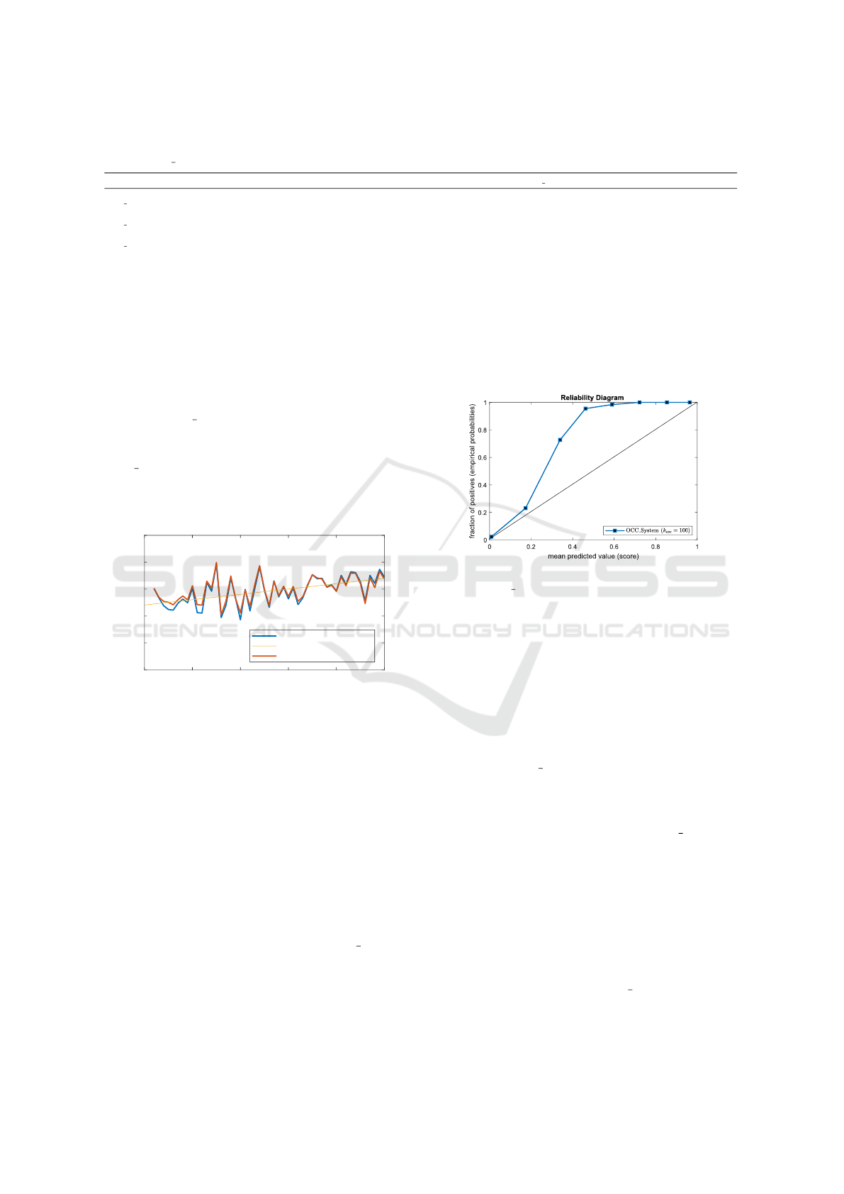
Table 1: Performance evaluation for several experiments (averaged on five runs) conducted with various versions of the GMM
and the OCC System. In brackets are reported the standard deviations.
Class. type k k
emb
Accuracy TPR FPR Specificity Precision F Score AUC IFM Brier Log loss
OCC Syst. (k
occ
= 15)
/ / 0.9718 0.9552 0.0153 0.9847 0.9803 0.9674 0.9884 0.9700 0.0410 0.2059
(0.0097) (0.0149) (0.0151) (0.0151 ) (0.0190) (0.0028) (0.0050) (0.0095) (0.0131) (0.0427)
OCC Syst. (k
occ
= 30)
/ / 0.9838 0.9747 0.0090 0.9910 0.9885 0.9814 0.9947 0.9829 0.0238 0.1779
(0.0058) (0.0155) (0.0063) (0.0063) (0.0080) (0.0068) (0.0102) (0.0067) (0.0059) (0.2037)
OCC Syst. (k
occ
= 100)
/ / 0.9824 0.0094 0.9772 0.9905 0.9938 0.9855 0.9958 0.9839 0.0302 0.1892
(0.0033) (0.0043) (0.0035) (0.0043) (0.0028) (0.0028) (0.0014) (0.0034) (0.0047) (0.0453)
GMM S
vs
Σ
sh
5.8 42.8 0.9453 0.9758 0.0852 0.9147 0.9038 0.9369 0.6370 0.9453 0.3130 19.4013
(1.3) (11.4) (0.01984) (0.02165) (0.06016) (0.06016) (0.06207) (0.0238) (0.0865) (0.0198) (0.0510) (0)
GMM S
vs
Σ
sh
-best 7 23 0.9668 0.9425 0.0090 0.9910 0.9880 0.9647 0.6375 0.9668 0.3249 19.4013
GMM S
vs
Σ
not−sh
15.2 9.4 0.7401 0.8103 0.3300 0.6700 0.6601 0.7255 0.5258 0.7401 0.4477 19.4013
(1.3) (6.9) (0.0134) (0.0578) (0.0696) (0.0696) (0.0345) (0.0125) (0.0766) (0.0134) (0.0114) (0)
GMM S
vs
Σ
not−sh
-best 16 5 0.7603 0.8391 0.3184 0.6816 0.6728 0.7468 0.4281 0.7603 0.4536 19.4013
GMM (BIC) Σ
sh
19.4, 20 34.8 0.8645 0.8379 0.1148 0.8852 0.8554 0.8436 0.5166 0.8616 0.4551 19.4013
(0.8), (0) (91.2) (0.0029) (0.0084) (0.0050) (0.0050) (0.0063) (0.0044) (0.0506) (0.0031) (0.0012) (0)
GMM (BIC) Σ
sh
-best 20, 20 40 0.9093 0.8793 0.0673 0.9327 0.9107 0.8947 0.7750 0.9060 0.3980 19.4013
GMM (BIC) Σ
not−sh
)
10.2, 7.2 4.6 0.6851 0.4908 0.1632 0.8368 0.7085 0.5669 0.5354 0.6638 0.4002 19.4013
(2.7), (0.7) (0.8) (0.0022) (0.0224) (0.0052) (0.0052) (0.0032) (0.0120) (0.0116) (0.0031) (0.0001) (0)
GMM (BIC) Σ
not−sh
)-best 8, 8 5 0.7632 0.6897 0.1794 0.8206 0.7500 0.7186 0.4359 0.7551 0.4062 19.4013
best ones, within the five runs, are provided. As con-
cerns the OCC System k
occ
= {15,30,100} are ex-
perimented. In terms of accuracy and informedness,
best performances (accuracy=98%) are reached by
OCC System for a structural complexity of the model
obtained with k
occ
= 30 clusters. Experiments with
k
occ
= 100 clusters do not show remarkable improve-
ments. As concerns GMM models, the configuration
0 10 20 30 40 50
embedding dimension
0
0.2
0.4
0.6
0.8
1
Performance
avg Accuracy
avg linear fitting (Accuracy)
avg Informedness
Figure 1: Average accuracy and informedness for the GMM
(shared covariance) as function of the embedding dimen-
sion k
emb
, measured on the test set S
ts
.
that reached comparable average performances (accu-
racy=94%) is the one with shared covariance, where
the hyper-parameters are obtained adopting a valida-
tion set S
vs
, with a low average number of compo-
nents k = 5.8 and an embedding dimension of k
emb
=
42.8. The worst experimented results, with an av-
erage accuracy of 68%, are achieved with a GMM
model with no shared covariance matrix, where the
model complexity (i.e. the number of components
k) is optimized through the BIC criterion. In sum-
mary, in terms of classification performances, results
are slightly different in favor of the OCC System,
even if the GMM does its best with a lower model
complexity, measured as the number of components
k. In Fig. 1 is reported the average accuracy and
informedness as function of the embedding dimen-
Figure 2: Reliability diagram for the score values s obtained
from the OCC System on the test set S
ts
.
sion k
emb
, measured on the test set S
ts
. Performances
varies widely with k
emb
. As expected, a great vari-
ability is found even in single experiments due to the
well-known strong dependence to initial conditions of
the EM algorithm. As concerns the calibration status
of the output classifiers, the Brier score and Log-Loss
– see Tab. 1 – show that both techniques needs cal-
ibration. For example, in Fig. 2 is depicted the Re-
liability diagram for the output probabilities obtained
through the OCC System. It confirms that the Reli-
ability curve is very far from the bisector line, indi-
cating that output score values are uncalibrated. The
same is confirmed by the calibration performances re-
ported in Tab. 1. Specifically, the OCC System is
found more reliable than the GMM in terms of Brier
score.
5 CONCLUSIONS
A comparison between some versions of the GMM
classification algorithm, able to operate in real val-
ued vector domains, and the OCC System, that works
with a custom-based weighted dissimilarity measure,
shows that remarkable performances can be obtained
Classification and Calibration Techniques in Predictive Maintenance: A Comparison between GMM and a Custom One-Class Classifier
509

choosing the right embedding for the first one. It is
well known that the perfect ML model does not exist
because each one possesses its own peculiar charac-
teristics. In our case the EM algorithm is fast and
the best GMM model obtained on the current ACEA
data set has a low computational complexity in terms
of the number of components, working with a shared
covariance matrix. As concerns the OCC System, it
reaches very good results in terms of accuracy, yield-
ing also classification models characterized by a low
number of clusters, even if the evolutionary procedure
slows down the training process. It is the price for ob-
taining a robust model where the weights of the cus-
tom based dissimilarity measures can be also inter-
preted as the importance of each feature in the clas-
sification task. This interesting feature, together with
clusters content analysis, allows knowledge discov-
ery applications. Moreover, some applications require
calibrated probabilities as output scores and both the
compared techniques show a weak calibration degree.
Future works will be grounded on the study and on the
application of several classical and newly proposed
calibration techniques for OCC System output scores,
as requested by the objectives of the main project.
ACKNOWLEDGEMENTS
The authors wish to thank ACEA Distribuzione
S.p.A. for providing the data and for their continu-
ous support during the design and test phases. Spe-
cial thanks to Ing. Stefano Liotta, Chief Network Op-
eration Division, to Ing. Silvio Alessandroni, Chief
Electric Power Distribution, and to Ing. Maurizio
Paschero, Chief Remote Control Division.
REFERENCES
ACEA (2014). The acea smart grid pilot project (in italian).
Akaike, H. (1974). A new look at the statistical model
identification. In Selected Papers of Hirotugu Akaike,
pages 215–222. Springer.
Bella, A., Ferri, C., Hern
´
andez-Orallo, J., and Ram
´
ırez-
Quintana, M. J. (2010). Calibration of machine learn-
ing models. In Handbook of Research on Machine
Learning Applications and Trends: Algorithms, Meth-
ods, and Techniques, pages 128–146. IGI Global.
Bellet, A., Habrard, A., and Sebban, M. (2013). A survey
on metric learning for feature vectors and structured
data. CoRR, abs/1306.6709.
Bianchi, F., De Santis, E., Rizzi, A., and Sadeghian, A.
(2015). Short-term electric load forecasting using
echo state networks and pca decomposition. Access,
IEEE, 3:1931–1943.
Brier, G. W. (1950). Verification of forecast expressed
in terms of probability. Monthly Weather Review,
78(1):1–3.
Cai, Y. and Chow, M.-Y. (2009). Exploratory analysis of
massive data for distribution fault diagnosis in smart
grids. In 2009 IEEE Power & Energy Society General
Meeting, pages 1–6. IEEE.
Cortes, C. and Vapnik, V. (1995). Support-vector networks.
Machine learning, 20(3):273–297.
De Santis, E., Livi, L., Sadeghian, A., and Rizzi, A. (2015).
Modeling and recognition of smart grid faults by a
combined approach of dissimilarity learning and one-
class classification. Neurocomputing, 170:368 – 383.
De Santis, E., Martino, A., Rizzi, A., and Mascioli, F. M. F.
(2018a). Dissimilarity space representations and auto-
matic feature selection for protein function prediction.
In 2018 International Joint Conference on Neural Net-
works (IJCNN), pages 1–8. IEEE.
De Santis, E., Paschero, M., Rizzi, A., and Mascioli,
F. M. F. (2018b). Evolutionary optimization of
an affine model for vulnerability characterization in
smart grids. In 2018 International Joint Conference
on Neural Networks (IJCNN), pages 1–8. IEEE.
De Santis, E., Rizzi, A., and Sadeghian, A. (2017a). A
learning intelligent system for classification and char-
acterization of localized faults in smart grids. In 2017
IEEE Congress on Evolutionary Computation (CEC),
pages 2669–2676.
De Santis, E., Rizzi, A., and Sadeghian, A. (2018c). A
cluster-based dissimilarity learning approach for lo-
calized fault classification in smart grids. Swarm and
evolutionary computation, 39:267–278.
De Santis, E., Rizzi, A., Sadeghian, A., and Mascioli, F.
(2013). Genetic optimization of a fuzzy control sys-
tem for energy flow management in micro-grids. In
IFSA World Congress and NAFIPS Annual Meeting
(IFSA/NAFIPS), 2013 Joint, pages 418–423.
De Santis, E., Sadeghian, A., and Rizzi, A. (2017b). A
smoothing technique for the multifractal analysis of a
medium voltage feeders electric current. International
Journal of Bifurcation and Chaos, 27(14):1750211.
DeGroot, M. H. and Fienberg, S. E. (1983). The com-
parison and evaluation of forecasters. Journal of the
Royal Statistical Society. Series D (The Statistician),
32(1/2):12–22.
Dempster, A. P., Laird, N. M., and Rubin, D. B. (1977).
Maximum likelihood from incomplete data via the em
algorithm. Journal of the Royal Statistical Society:
Series B (Methodological), 39(1):1–22.
Duin, R. P., Pe¸kalska, E., and Loog, M. (2013). Non-
euclidean dissimilarities: causes, embedding and in-
formativeness. In Similarity-Based Pattern Analysis
and Recognition, pages 13–44. Springer.
Guikema, S. D., Davidson, R. A., and Liu, H. (2006). Statis-
tical models of the effects of tree trimming on power
system outages. IEEE Transactions on Power Deliv-
ery, 21(3):1549–1557.
Khan, S. S. and Madden, M. G. (2010). A survey of recent
trends in one class classification. In Coyle, L. and
CI4EMS 2020 - Special Session on Computational Intelligence for Energy Management and Storage
510

Freyne, J., editors, Artificial Intelligence and Cogni-
tive Science, volume 6206 of Lecture Notes in Com-
puter Science, pages 188–197. Springer Berlin Hei-
delberg.
Kuleshov, V., Fenner, N., and Ermon, S. (2018). Accurate
uncertainties for deep learning using calibrated regres-
sion. arXiv preprint arXiv:1807.00263.
Liu, H., Davidson, R. A., Rosowsky, D. V., and Stedinger,
J. R. (2005). Negative binomial regression of electric
power outages in hurricanes. Journal of infrastructure
systems, 11(4):258–267.
Martino, A., De Santis, E., Baldini, L., and Rizzi, A. (2019).
Calibration techniques for binary classification prob-
lems: A comparative analysis. In Proceedings of
the 11th International Joint Conference on Computa-
tional Intelligence, volume 1 of IJCCI2019.
M
¨
uller, M. (2007). Dynamic time warping. Information
retrieval for music and motion, pages 69–84.
Murphy, A. H. and Winkler, R. L. (1977). Reliability of sub-
jective probability forecasts of precipitation and tem-
perature. Journal of the Royal Statistical Society. Se-
ries C (Applied Statistics), 26(1):41–47.
Pe¸kalska, E. and Duin, R. (2005). The dissimilarity rep-
resentation for pattern recognition: foundations and
applications. Series in machine perception and artifi-
cial intelligence. World Scientific.
Possemato, F., Paschero, M., Livi, L., Rizzi, A., and
Sadeghian, A. (2016). On the impact of topological
properties of smart grids in power losses optimization
problems. International Journal of Electrical Power
& Energy Systems, 78:755–764.
Schwarz, G. et al. (1978). Estimating the dimension of a
model. The annals of statistics, 6(2):461–464.
Storti, G. L., Paschero, M., Rizzi, A., and Mascioli, F.
M. F. (2015). Comparison between time-constrained
and time-unconstrained optimization for power losses
minimization in smart grids using genetic algorithms.
Neurocomputing, 170:353–367.
Wang, Z. and Zhao, P. (2009). Fault location recogni-
tion in transmission lines based on support vector ma-
chines. In 2009 2nd IEEE International Conference
on Computer Science and Information Technology,
pages 401–404. IEEE.
Zhang, Y., Huang, T., and Bompard, E. F. (2018). Big data
analytics in smart grids: a review. Energy informatics,
1(1):8.
Classification and Calibration Techniques in Predictive Maintenance: A Comparison between GMM and a Custom One-Class Classifier
511