Complexity vs. Performance in Granular Embedding Spaces for Graph

Classiﬁcation

Luca Baldini

, Alessio Martino

and Antonello Rizzi

Department of Information Engineering, Electronics and Telecommunications, University of Rome “La Sapienza”,

via Eudossiana 18, 00184 Rome, Italy

Keywords:

Structural Pattern Recognition, Supervised Learning, Embedding Spaces, Granular Computing, Graph Edit

Distances.

Abstract:

The most distinctive trait in structural pattern recognition in graph domain is the ability to deal with the

organization and relations between the constituent entities of the pattern. Even if this can be convenient and/or

necessary in many contexts, most of the state-of the art classiﬁcation techniques can not be deployed directly

in the graph domain without ﬁrst embedding graph patterns towards a metric space. Granular Computing is a

powerful information processing paradigm that can be employed in order to drive the synthesis of automatic

embedding spaces from structured domains. In this paper we investigate several classiﬁcation techniques

starting from Granular Computing-based embedding procedures and provide a thorough overview in terms of

model complexity, embedding space complexity and performances on several open-access datasets for graph

classiﬁcation. We witness that certain classiﬁcation techniques perform poorly both from the point of view

of complexity and learning performances as the case of non-linear SVM, suggesting that high dimensionality

of the synthesized embedding space can negatively affect the effectiveness of these approaches. On the other

hand, linear support vector machines, neuro-fuzzy networks and nearest neighbour classiﬁers have comparable

performances in terms of accuracy, with second being the most competitive in terms of structural complexity

and the latter being the most competitive in terms of embedding space dimensionality.

1 INTRODUCTION

The possibility of solving pattern recognition prob-

lems in the graph domain challenged computer sci-

entists and machine learning engineers alike for more

than two decades. That is because graphs are able

to encode both topological information (namely, re-

lationship between entities) and semantic information

(whether nodes and/or edges are equipped with suit-

able attributes). In turn, this high level of abstrac-

tion and customization made graphs suitable mathe-

matical objects for modelling several real-world sys-

tems in ﬁelds such as biology, social networks anal-

ysis, computer vision and image analysis. The draw-

back when dealing with graph-based pattern recogni-

tion relies on the computational complexity required

in order to measure the (dis)similarity between two

graphs, which exponentially grows with respect to

their size (Bunke, 2003). This inevitably results in

https://orcid.org/0000-0003-4391-2598

https://orcid.org/0000-0003-1730-5436

https://orcid.org/0000-0001-8244-0015

an heavy computational burden when it comes to per-

form pattern recognition in the graph domain, espe-

cially when also node and/or edge attributes have to

be taken into account.

One of the mainstream approaches when dealing

with graph-based pattern recognition relies on embed-

ding spaces: in short, the pattern recognition problem

is cast from the structured input domain towards the

Euclidean space in which classiﬁcation is performed.

Nonetheless, building the embedding space is a deli-

cate issue that must ﬁll the informative and semantic

gap between the two domains (Baldini et al., 2019a).

This paper follows two previous works (Baldini

et al., 2019a; Baldini et al., 2019b) on the deﬁnition

of embedding spaces for graph classiﬁcation thanks

to the Granular Computing paradigm (Bargiela and

Pedrycz, 2006; Bargiela and Pedrycz, 2003; Pedrycz,

2001). According to the latter, structured domains

can be analyzed by means of suitable information

granules, namely small data aggregates that endow

similar functional and/or structural characteristics.

Speciﬁcally, we investigate several classiﬁcation sys-

338

Baldini, L., Martino, A. and Rizzi, A.

Complexity vs. Performance in Granular Embedding Spaces for Graph Classiﬁcation.

DOI: 10.5220/0010109503380349

In Proceedings of the 12th International Joint Conference on Computational Intelligence (IJCCI 2020), pages 338-349

ISBN: 978-989-758-475-6

tems working on a properly-synthesized embedding

space. In fact, in our previous works (Baldini et al.,

2019a; Baldini et al., 2019b) we used a plain nearest

neighbours decision rule for the sake of simplicity.

Notwithstanding that, a nearest neighbours decision

rule suffers from several drawbacks, including high

computational burden, sensitivity to the classes distri-

bution and the number of classes. Hence, in this work,

we consider ﬁve different classiﬁers operating in the

embedding space: two support vector machines vari-

ants (with linear and radial basis kernels), two neuro-

fuzzy approaches and K-nearest neighbours. We pro-

vide a general three-fold overview in terms of perfor-

mances, embedding space complexity and structural

complexity of the adopted classiﬁcation system.

The remainder of this paper is structured as fol-

lows: in Section 2 we provide an overview of possible

strategies for solving pattern recognition problems in

structured domains, with a major emphasis on Granu-

lar Computing-based systems; in Section 3 we intro-

duce GRALG, the Granular Computing-based graph

classiﬁcation system at the basis of this work; in Sec-

tion 4 we introduce the datasets used for analysis,

along with the proper computational results; ﬁnally,

Section 5 concludes the paper.

2 CURRENT APPROACHES FOR

PATTERN RECOGNITION ON

THE GRAPH DOMAIN

In the literature, several mainstream strategies can

be found in order to solve pattern recognition prob-

lems in structured domains. According to the macro-

taxonomy presented in (Martino et al., 2018a), ﬁve

main strategies can be found. A ﬁrst strategy consists

in engineering numerical features to be drawn from

the structured data at hand, to be concatenated in a

vector form. Examples of feature engineering tech-

niques involve entropy measures (Han et al., 2011;

Ye et al., 2014; Bai et al., 2012), centrality measures

(Mizui et al., 2017; Martino et al., 2018b; Leone Scia-

bolazza and Riccetti, 2020; Martino et al., 2020a),

heat trace (Xiao and Hancock, 2005; Xiao et al.,

2009) and modularity (Li, 2013). Whilst this ap-

proach is straightforward and allows to move the pat-

tern recognition problem towards the Euclidean space

in which any pattern recognition algorithm can be

used without alterations, designing the mapping func-

tion (i.e., enumerating the set of numerical features to

be extracted) requires a deep knowledge of both the

problem and the data at hand: indeed, the input spaces

being equal, speciﬁc subsets of features allow to solve

different problems.

A dual strategy consists in deﬁning ad hoc dissim-

ilarity measures tailored to the input space under anal-

ysis. In this manner, the pattern recognition problem

can directly be solved in the input space without any

explicit cast towards the Euclidean space. On the plus

side, the input space might not be metric altogether,

yet this is not a prerogative; on the negative side, this

limits the range of pattern recognition algorithms that

can be employed. Indeed, the possibility of the input

space being non-metric reﬂects the non-metric pecu-

liarity of the dissimilarity measure itself: as such, the

pattern recognition algorithm must not rely on any

algebraic structures (e.g., mean, median, inner prod-

uct) and leverage pairwise dissimilarities only. Ex-

amples of custom dissimilarity measures include the

so-called edit distances, deﬁned both on graph (Bal-

dini et al., 2019a; Baldini et al., 2019b) and sequence

(Levenshtein, 1966; Cinti et al., 2020) domains.

A further family is composed by embedding tech-

niques, which can either be explicit or implicit.

Amongst the implicit embedding techniques, ker-

nel methods emerge (Schölkopf and Smola, 2002;

Shawe-Taylor and Cristianini, 2004): kernel methods

exploit the so-called kernel trick (i.e., the inner prod-

uct in a reproducing kernel Hilbert space) in order

to measure similarity between patterns. In the litera-

ture, have been proposed several graph kernels (Kon-

dor and Lafferty, 2002; Borgwardt and Kriegel, 2005;

Shervashidze et al., 2009; Shervashidze and Borg-

wardt, 2009; Vishwanathan et al., 2010; Shervashidze

et al., 2011; Livi and Rizzi, 2013; Neumann et al.,

2016; Ghosh et al., 2018; Bacciu et al., 2018) that,

for example, consider substructures such as (random)

walks, trees, paths, cycles in order to measure simi-

larity or exploit propagation/diffusion schemes. Con-

versely, as explicit embedding techniques are con-

cerned, dissimilarity spaces are one of the main ap-

proaches (P˛ekalska and Duin, 2005). A dissimilar-

ity space can be built by ﬁrst deﬁning an ad-hoc dis-

similarity measure and then evaluating the pairwise

dissimilarity matrix which can be considered as em-

bedded in a Euclidean space: in other words, each

original (structured) pattern is represented by a real-

valued vector containing the distances with respect to

all other patterns (P˛ekalska and Duin, 2005) or with

respect to a properly selected subset of prototypes

(P˛ekalska et al., 2006). Alongside embedding meth-

ods, deep learning approaches are emerging as effec-

tive frameworks for different tasks like graph classiﬁ-

cation, link prediction and node classiﬁcation (Zhang

et al., 2019; Wu et al., 2020). In this context, the neu-

ral architectures typically implement a convolution

layer resembling the well-know convolutional neural

Complexity vs. Performance in Granular Embedding Spaces for Graph Classiﬁcation

339

networks, with the scope to learn nodes representa-

tion taking into account neighbours features. Two

distinct approaches are typically employed: spectral-

based methods perform convolution operation in the

spectral domain by means of Graph Fourier Trans-

form (Kipf and Welling, 2016; Bianchi et al., 2019),

whilst spatial-based approaches used to aggregates

nodes attributes by directly exchanging information

amongst neighbours (Niepert et al., 2016; Hamilton

et al., 2017).

As anticipated in Section 1, Granular Comput-

ing is a powerful information processing paradigm

for building explicit embedding spaces and has been

successfully applied for synthesizing effective and in-

terpretable advanced pattern recognition systems for

structured data (see e.g. (Rizzi et al., 2012; Baldini

et al., 2019a; Baldini et al., 2019b; Martino et al.,

2019a; Martino et al., 2020b; Bianchi et al., 2014a;

Bianchi et al., 2014b; Bianchi et al., 2016) and ref-

erences therein). In short, Granular Computing is of-

ten described as a human-centered information pro-

cessing paradigm based on formal mathematical en-

tities known as information granules (Bargiela and

Pedrycz, 2006). The human-centered computational

concept in soft computing and computational intel-

ligence was initially developed by Lotﬁ A. Zadeh

through fuzzy sets (Zadeh, 1979) that exploits human-

inspired approaches to deal with uncertainties and

complexities in data. The process of ‘granulation’,

intended as the extraction of meaningful aggregated

data, mimics the human mechanism needed to or-

ganize complex data from the surrounding environ-

ment in order to support decision making activities

and to describe the world around (Pedrycz, 2016). For

this reason, Granular Computing can be described as

a framework for analyzing data in complex systems

aiming to provide human interpretable results (Mar-

tino et al., 2020b). The importance of information

granules resides in the ability to underline properties

and relationships between data aggregates. Speciﬁ-

cally, their synthesis can be achieved by following the

indistinguishability rule, according to which elements

that show enough similarity, proximity or functional-

ity shall be grouped together (Zadeh, 1997; Pedrycz

and Homenda, 2013). With this approach, each gran-

ule is able to show homogeneous semantic informa-

tion from the problem at hand. Furthermore, data

at hand can be represented using different levels of

‘granularity’ and thus different peculiarities of the

considered system can emerge. Depending on this

resolution, an unknown computational process to be

modelled may exhibit different properties and differ-

ent atomic units that show different representations

of the system as a whole. Clearly, an efﬁcient and

automatic procedure to select the most suitable level

of abstraction according to both the problem at hand

and the data description is of utmost importance. Due

to the tight link between ‘information granules’ and

‘groups of similar data’, the most straightforward ap-

proach in order to synthesize a possibly meaning-

ful set of information granules can be found in data

clustering (Frattale Mascioli et al., 2000; Pedrycz,

2005; Ding et al., 2015). Since the clustering proce-

dure is usually employed to discover groups of sim-

ilar data aggregates, it operates in the input (struc-

tured) domain: to this end, not only the (dis)similarity

measure, but also the cluster representative shall be

tailored accordingly. In order to represent clusters

in structured domains, the medoid (also called Min-

SOD) is usually employed (Martino et al., 2019b),

due to the fact that its evaluation relies only on pair-

wise dissimilarities between patterns belonging to the

cluster itself, without any algebraic structures that can

not be deﬁned in non-geometric spaces. The clus-

ter representatives from the resulting partition can

be considered as symbols belonging to an alphabet

A = {s

, ..., s

}: these symbols are the pivotal gran-

ules on the top of which the embedding space can

be built thanks to the symbolic histograms paradigm.

According to the latter, each pattern can be described

as an n-length integer-valued vector which counts in

position i the number of occurrences of the i

symbol

drawn from the alphabet within the patter itself. The

embedding space can ﬁnally be equipped with alge-

braic structures such as the Euclidean distance or the

dot product and standard classiﬁcation systems can be

used without alterations.

3 GRALG

The classiﬁcation system considered in this work

is called GRALG (GRanular computing Approach

for Labeled Graphs) originally proposed in (Bianchi

et al., 2014a). GRALG aims to be a general purpose

classiﬁer for labelled graphs embracing the Granular

Computing paradigm. The main core of the classi-

ﬁer is a graph embedding procedure via symbolic his-

tograms, the geometric representation of graphs built

upon the symbols in an alphabet A which, in turn,

are synthesized in an unsupervised way through an

ensemble of clustering algorithms. These two stages

rely on a suitable dissimilarity measure, which al-

lows the pattern comparison in the graph domain. In

this section, we ﬁrst introduce the dissimilarity mea-

sure involved in the atomic operations between graphs

(Section 3.1) and then we provide a brief description

of the building blocks that make up the stages needed

NCTA 2020 - 12th International Conference on Neural Computation Theory and Applications

340

to perform the explicit graph mapping towards a suit-

able embedding space (Sections 3.2–3.5), along the

way in which they cooperate for training (Section 3.6)

and testing (Section 3.7) the overall system.

3.1 Graph Edit Distance

As anticipated in Section 2, the Graph Edit Distance

(GED) is a common approach to evaluate the dissim-

ilarity between graphs. GEDs deﬁne the distance be-

tween two graph G

and G

as the minimum cost

path needed to turn G

into G

, by applying a se-

ries of atomic operations deﬁned on both vertices and

edges: substitution, insertion and deletion. Besides

the costs, the edit operations may also be associated

to some weights in order to reﬂect the importance

of the aforementioned operations. Generally speak-

ing, the dissimilarity measure d : G ×G → R between

two graphs can be cast as the following minimization

problem:

d(G

, G

) = min

(ε

,...,ε

)∈O(G

)

∑

i=1

c(ε

) (1)

where c (ε

) is the cost associated to the generic

edit

operation ε

and O(G

, G

) is the set of prospective

operations that gives an isomorphism between the two

graphs. The main drawback when using a GED is the

unfeasible computational complexity needed to com-

pute an exact solution of Eq. (1) and, for this reason,

many heuristics were proposed in order to solve the

graph matching problem in a sub-optimal manner, yet

with reasonable computational burden. Given these

aspects, in GRALG we employ a greedy heuristic

called node Best Match First (nBMF) (Bianchi et al.,

2016) in order to measure the dissimilarity between

graphs. Formally, let G

= (V

, E

, L

) and G

, E

, L

) be two graphs labelled on both edges

and vertices. Furthermore, let d

: L

× L

→ R and

: L

× L

→ R be the dissimilarities deﬁned on

nodes’ and edges’ attributes (L

and L

, respectively).

For the sake of generalization, d

and d

might be

parametric with respect to π

and π

, namely sets of

real-valued parameters required to evaluate d

and

, respectively. In nBMF, the substitution cost on

nodes and edges is evaluated with the corresponding

dissimilarity function (d

and d

). Accordingly, it

is possible to deﬁne the overall substitution costs on

nodes and edges (c

sub

nodes

and c

sub

edge

) by summing up the

dissimilarity values of all the nodes or edges substi-

tuted during the procedure. Conversely, insertion and

deletion costs c

ins

node

, c

ins

edge

, c

del

node

, c

del

edge

depend on the

difference between the two graphs in terms of nodes

Regardless on whether it is a substitution, deletion or

insertion on nodes or edges.

and edges set cardinality. The interested reader can

found detailed pseudo-codes describing the nBMF in

(Baldini et al., 2019a). Additionally, each operation

is weighted by w

sub

node

, w

sub

edge

, w

ins

node

, w

ins

edge

, w

del

node

, w

del

edge

individually bounded in [0, 1]. At the end of the pro-

cedure, the dissimilarities between nodes and edges,

say d

, V

) and d

, E

), are evaluated as:

, V

) = w

sub

node

sub

node

+ w

ins

node

ins

node

+ w

del

node

del

node

, E

) = w

sub

edge

sub

edge

+ w

ins

edge

ins

edge

+ w

del

edge

del

edge

(2)

Each dissimilarity is normalized by taking into ac-

count the different orders between the two graphs:

, V

) =

, V

)

max{o

, o

}

, E

) =

, E

)

(min{o

, o

} · (min{o

, o

} − 1))

(3)

with o

= |V

| and o

= |V

|. Finally, the dissimilar-

ity between the two graphs reads as:

d(G

, G

) =



, V

) + d

, E

)



(4)

3.2 Extractor

The subgraph extraction block aims at breaking down

a graph into its constituent parts following a stochas-

tic subsampling approach operating in a class-aware

fashion. These improvements have been thoroughly

described and tested in (Baldini et al., 2019a) and

(Baldini et al., 2019b), to which the interested reader

is referred to for further details, in order to overcome

the main limitation of GRALG: indeed, in its origi-

nal implementation (Bianchi et al., 2014a), GRALG

used to exhaustively extract all subgraphs up to a

given user-deﬁned order o from any input graph, re-

sulting in a non-negligible running time and memory

footprint. In (Baldini et al., 2019a), we show how a

stochastic subsampling can lead to comparable per-

formances with respect to the original (exhaustive)

implementation with remarkably lower running times

and memory usage. Indeed, this procedure builds a

subgraph set with a ﬁxed cardinality W by extract-

ing subgraphs uniformly at random (replacements are

allowed) from a set of graphs using either one of

two well-known traversal strategies, namely Breadth

First Search and Depth First Search. Furthermore, in

(Baldini et al., 2019b), we show how the stochastic

subsampling granulation procedure can be performed

in a class-aware fashion: this allows the exploita-

tion of the ground-truth class labels in the training

data, resulting in a more effective alphabet synthe-

sis. The latter, being competitive both in terms of per-

Complexity vs. Performance in Granular Embedding Spaces for Graph Classiﬁcation

341

formances and computational complexity, is the strat-

egy we used in this work. Let S be a set of graphs,

each of which is associated to its ground-truth class

label L with L ∈ {1, . . . , N} and N being the number

of classes. The class-aware stochastic extraction ran-

domly draws a graph G := {V , E} from S and then

randomly draws a vertex v ∈ V . Then, starting from

the node v, a suitable traversal strategy explores G

collecting a subgraph g = {V

, E

} with V

⊂ V ver-

tices and E

⊂ E edges. The subgraph g is inserted

in a subgraph set S

according to the graph’s label L.

In this way, it is also possible to the deﬁne the num-

ber of subgraphs W to be sampled from the starting

set by ﬁxing how many times the procedure must oc-

cur, since each extraction outputs a single graph. The

maximum order o of the extracted subgraph, namely

the maximum number of vertices for all subgraphs g,

is still a user-deﬁned parameter. Conversely to the

original work (Bianchi et al., 2014a), this procedure

allows to arbitrary choose the cardinality W of the

subgraphs set

L=1

and consequently relieves the

memory issues and improves the wall-clock runtime

of the algorithm.

3.3 Granulator

The Granulator deﬁnes a procedure able to synthe-

size information granules by building the alphabet

A = {s

, . . . , s

}, namely a set that collects the rele-

vant substructures s

starting from a given subgraphs

set. The core method in charge of returning suit-

able information granules is the Basic Sequential Al-

gorithmic Scheme (BSAS) clustering algorithm (Bal-

dini et al., 2019a; Baldini et al., 2019b) that works

directly in the graph domain thanks to the dissimilar-

ity measure described in Section 3.1. BSAS needs

two parameters: the dissimilarity threshold θ below

which a pattern is included into the closest cluster and

the maximum number of allowed clusters Q, in or-

der to reasonably bound the number of resulting clus-

ters which can grow indeﬁnitely (especially for small

values of θ). According to the Granular Computing

paradigm, the granulator shall extract symbols by ex-

ploring different levels of abstraction for the problem

at hand: indeed, the granulation performs a clustering

ensemble procedure by generating different partitions

of the input data using different θ values. Then, for

every cluster C in the resulting partitions, a cluster

quality index F(C) is deﬁned as:

F(C) = η · Φ(C) + (1 − η) · Θ(C) (5)

where the two terms Φ(C) and Θ(C) are respectively

the compactness and the cardinality of cluster C, de-

ﬁned in turn as:

Φ(C) =

|C| − 1

∑

d(g

∗

, g

) (6)

Θ(C) = 1 −

|C|

(7)

where g

∗

is the representative of cluster C and g

the

pattern in the cluster. In this way, we evaluate each

cluster by considering its compactness Φ and cardi-

nality Θ, whose importance is weighted by a trade-off

parameter η ∈ [0, 1]. Since the BSAS operates in the

graph domain, as discussed in Section 2, the repre-

sentative g

∗

is deﬁned as the medoid of the cluster,

namely the element that minimizes the pairwise sum

of distances among all patterns in the cluster (Martino

et al., 2019b). Finally, by thresholding F(C) with

a value τ

, only well-formed clusters (i.e., compact

and populated) are promoted to be symbols s belong-

ing to the alphabet A. Since the symbol synthesis oc-

curs on a labelled training set and since the Extrac-

tor operates in a class-aware fashion (Section 3.2),

the clustering ensemble is performed individually on

the S

sets, hence collecting class-related symbols in

class-aware alphabets A

, which are ﬁnally merged

together in A =

L=1

3.4 Embedder

The Embedder block plays the key role necessary to

map patterns from the graph domain towards a ge-

ometric (Euclidean) space. Formally, let G be the

graph domain, the Embedder is in charge of build-

ing the function φ : G → D that maps the graph do-

main into an n-dimensional space D ⊆ R

. The em-

bedding function relies on the symbolic histograms

paradigm, exploiting the relevant substructures syn-

thesized by the Granulator (i.e., the alphabet). In or-

der to describe this process, let G

exp

be the set made

up of the subgraphs in G ∈ G, i.e. the expanded rep-

resentation of G in subgraphs. Given the alphabet set

A = {s

, . . . , s

}, the vectorial representation h (i.e.,

the symbolic histogram) of G is a vector whose com-

ponents represents the number of occurrences of each

symbol s ∈ A in G

exp

h = φ

exp

) = [occ(s

, G

exp

), . . . , occ(s

, G

exp

)]

(8)

The function occ : A → N compares a symbol s

with

j = 1 . . . n and all the subgraphs g ∈ G

exp

. If the

resulting dissimilarity measure is below a symbol-

dependent threshold value τ

= Φ(C

) · ε, this counts

as a match and the counter is increased by 1. The ε

value is a user-deﬁned tolerance parameter and C

the cluster whose MinSOD is s

. It is worth remark-

ing here that the computational complexity needed to

NCTA 2020 - 12th International Conference on Neural Computation Theory and Applications

342

expand exhaustively G in the set of its subgraph G

exp

may lead to memory issues, since the number of sub-

graphs grows exponentially with respect to the order

of graph. Furthermore, the number of matches needed

to build the embedding space can be very large since

all symbols have to be compared with the subgraphs

in G

exp

. This could lead to unfeasible running times

even for medium size datasets. For this reason, the set

exp

is evaluated with a deterministic algorithm that

tries to partially expand G = {V , E}: starting from

a seed node v ∈ V , the same traverse strategy em-

ployed in the Extractor drives the exploration and the

extraction of subgraphs from G, starting from order 1

up until a user-deﬁned value o and collects these sub-

structures in G

exp

. Since the goal of the procedure is

to limit the cardinality of G

exp

, if a node v ∈ V al-

ready appears in one of the previously-extracted sub-

graphs, it will not be eligible to be a seed node for

further traversals. The procedure goes on as long as a

vertex v ∈ V can be legally used as root node for the

traversal strategy.

3.5 Classiﬁer

The three blocks in Sections 3.2–3.4 allow us to build

an embedding space D ⊆ R

, where each graph is

mapped with an appropriate vector h ∈ D, i.e. its

symbolic histogram. Further, such approach allows

us to use any classiﬁer designed in R

without limita-

tions. In this work, we considered different classiﬁca-

tion systems:

Support Vector Machines (SVMs) aim at estimat-

ing the decision boundary between two classes by

a maximal-margin hyperplane. We employed the

well-known ν-SVM (Schölkopf et al., 2000) using

two different kernels: the linear kernel endowing

the dot product between patterns K (x, x

) = hx, x

and a non-linear radial basis function (RBF) ker-

nel, i.e. K (x, x

) = exp{−γkx − x

}

Neuro-Fuzzy Min-Max classiﬁer relying on the

construction of hyperboxes, which serve as

atomic geometric structures needed to deﬁne

the decision boundary in the training phase.

Speciﬁcally, we tested two algorithms for training

the model (i.e., building hyperboxes): Adaptive

Resolution Classiﬁer (ARC) and Pruning Adap-

tive Resolution Classiﬁer (PARC) (Rizzi et al.,

2002).

K-Nearest Neighbours (K-NN) in which, when an

unseen pattern is considered for classiﬁcation, its

K nearest patterns are selected and the decision is

taken according to the most voted class amongst

the K patterns (Cover and Hart, 1967).

3.6 Training Phase

After individual and detailed descriptions of the build-

ing blocks that made up the GRALG classiﬁcation

system, here we describe how those blocks cooper-

ate together in order to synthesize the ﬁnal model. To

this end, let S be a dataset of labelled graphs on nodes

and/or edges and let S

, S

and S

be the training,

validation and test set drawn from S:

Extractor: takes as input S

and the parameter W

and, according to the description given in Section

3.2, extracts N different class-speciﬁc subgraphs

sets S

g,tr

Granulator: each class-aware subgraphs set S

g,tr

granulated and consequently A

class-speciﬁc al-

phabets are constructed

Embedder: the overall alphabet A =

L=1

, with

n = |A| symbols, enters the embedding block.

First, all graphs in S

and S

are expanded as de-

scribed in Section 3.4. Then, for each G

∈ S

and G

∈ S

, we can construct the associated

vector representation h

∈ D and h

∈ D such

that D ⊆ R

Classiﬁer: given the embedded version of training

and validation set (h

and h

), the quality of

the mapping function is evaluated by considering

a given classiﬁer (amongst the ones presented in

Section 3.5) which is trained on h

and later eval-

uated on h

The procedures involved to complete a graph classi-

ﬁcation are very sensitive to speciﬁc parameters that

can strongly affect the overall performances. In or-

der to face this issue, two different optimizations take

place separately.

3.6.1 Alphabet Optimization Phase

A ﬁrst stage of optimization aims to synthesize an op-

timal set of symbols A

∗

and properly tune the hyper-

parameters of the chosen classiﬁer, by deploying an

evolutive strategy, i.e. a genetic algorithm. In order to

purse this goal, the following parameters (and corre-

sponding procedures) are considered:

GED: the dissimilarity measure in the graph domain

requires a ﬁne tuning of the 6 weights for the

edit operations: W = {w

sub

node

, w

sub

edge

, w

ins

node

, w

ins

edge

del

node

, w

del

edge

}. Depending on the dataset, both

vertices and edges can require a parametric dis-

similarity measure d

and d

with parameters

Π = {π

, π

} whose values are optimized as well.

Granulator: in order to synthesize an optimal alpha-

bet, we optimize Q (maximum number of allowed

Complexity vs. Performance in Granular Embedding Spaces for Graph Classiﬁcation

343

clusters for BSAS), τ

(MinSOD quality thresh-

old for being promoted to a symbol) and η (trade-

off parameter that weights compactness and car-

dinality in Eq. (5)).

Classiﬁer: the set of hyperparameters C that depends

on the considered classiﬁer:

• ν-SVM: only the regularization term ν ∈ (0, 1].

• RBF ν-SVM: along with ν ∈ (0, 1], we also

tune the kernel shape γ ∈ (0, 100].

• ARC/PARC: we optimize the λ ∈ (0, 1) pa-

rameter used as trade-off between the error on

training set and the network complexity. Fur-

thermore, we optimize the type of membership

function (to be chosen between Trapezoidal and

Simpson’s) and the decay parameter µ ∈ (0, 1)

associated with it.

• K-NN: the number K ∈ [1, 2

|] of nearest

patterns involved in the voting.

To summarize, the genetic code reads as:

[Q τ

η W Π C] (9)

whereas the ﬁtness function J

al ph

reads as the classi-

ﬁer accuracy ω ∈ [0, 1] on the validation set:

al ph

= ω(S

) =

∑

i=1

δ(y

, ˆy

)

(10)

with

δ(y

, ˆy

) =

(

1 if y

= ˆy

0 otherwise

(11)

and where, in turn, ˆy

and y

are (respectively) the pre-

dicted label and the ground-truth label for i-th pattern

in S

. Standard genetic operators (mutation, selec-

tion, crossover and elitism) take care of moving from

one generation to the next. The best individual is re-

tained at the end of the evolution, speciﬁcally the por-

tions of the genetic code W

and Π

, along with the

alphabet A

synthesized using its genetic code.

3.6.2 Feature Selection Phase

The cardinality of A

and consequently the embed-

ding space D ⊆ R

may be too large, impacting

the classiﬁcation performance and the interpretabil-

ity of the ﬁnal model. To this end, we implement

a feature selection phase still based on genetic opti-

mazation. Formally, let m ∈ {0, 1}

be a projection

mask, then:

1. we perform the component-wise product between

the mask and the embedded vectors of the training

set:

= m h

(12)

by further neglecting components corresponding

to 0’s in h

. Hence, it is possible to ﬁgure h

as lying in a (possibly) reduced embedding space

D ⊆ R

with m ≤ n

2. according to the mask m employed in step 1, the

validation set h

∈ D is reduced in the same way,

leading to h

∈ D

3. the classiﬁcation system is trained on h

using the

hyperparameters set C . The accuracy on the (re-

duced) validation set h

is ﬁnally computed.

Following this scheme, a genetic algorithm drives the

optimization of the mask m and, at the same time, the

classiﬁer hyperparameters C by maximizing a ﬁtness

function J

f s

that reads as the linear convex combina-

tion between the classiﬁer accuracy on the validation

set and the cost of the mask weighted by a trade-off

value α ∈ [0, 1]:

f s

= α ·ω (S

) + (1 − α) · µ (13)

where the cost of the mask µ ∈ [0, 1] is deﬁned as:

µ = 1 −

|{i : m

= 1}|

|m|

(14)

When the evolution is completed, the best individual

is retained, as it encodes the optimal projection mask

, able to return the reduced alphabet A

, and the

optimal set of parameters C

used to train the classi-

ﬁer in the embedding space D.

3.7 Synthesized Classiﬁcation Model

After the two optimizations stages are over, the ﬁnal

classiﬁcation performances can be evaluated on the

test set. First, the test set S

is embedded in the vec-

tor space D. To this aim, the embedder block specif-

ically equipped with parameters W

and Π

for the

GED dissimilarity measure, outputs the vector set h

by taking advantage of the alphabet A

. The classiﬁer

returned by the optimization phase (i.e., trained on the

projected vectors h

with the hyperparameters C

∗

) is

tested on the embedded test set h

∈ D, returning the

overall accuracy of the GRALG system.

4 EXPERIMENTS

Five different datasets from the IAM repository

(Riesen and Bunke, 2008) have been considered for

testing:

Letter: a triad of datasets where each graph repre-

sents a letter drawing with different level of distor-

tions: low (L), medium (M) and high (H). Match-

NCTA 2020 - 12th International Conference on Neural Computation Theory and Applications

344

AIDS GREC Letter-L Letter-M Letter-H

100

110

Accuracy [%]

(a) ARC

AIDS GREC Letter-L Letter-M Letter-H

100

110

Accuracy [%]

(b) PARC

AIDS GREC Letter-L Letter-M Letter-H

100

110

Accuracy [%]

AIDS GREC Letter-L Letter-M Letter-H

100

110

Accuracy [%]

(d) RBF ν-SVM

AIDS GREC Letter-L Letter-M Letter-H

100

110

Accuracy [%]

(e) K-NN

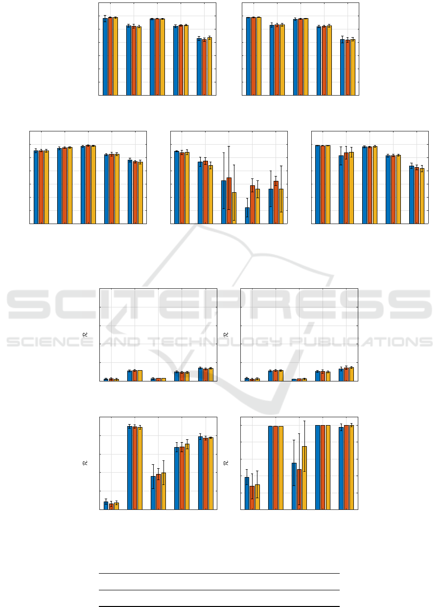
Figure 1: Accuracy comparison for the 5 classiﬁers. Blue, red and yellow bars correspond to subsampling rates W =

10%, 30%, 50%, respectively. Whiskers indicate the standard deviation.

AIDS GREC Letter-L Letter-M Letter-H

0.2

0.4

0.6

0.8

(a) ARC

AIDS GREC Letter-L Letter-M Letter-H

0.2

0.4

0.6

0.8

(b) PARC

AIDS GREC Letter-L Letter-M Letter-H

0.2

0.4

0.6

0.8

AIDS GREC Letter-L Letter-M Letter-H

0.2

0.4

0.6

0.8

(d) RBF ν-SVM

Figure 2: Complexity ratio for SVM and Min-Max classiﬁers. For bar legend, see caption of Fig. 1.

Table 1: Number of subgraphs extracted from S

(o = 5) by the exhaustive procedure.

Letter-L Letter-M Letter-H GREC AIDS

8193 8582 21165 27119 35208

Complexity vs. Performance in Granular Embedding Spaces for Graph Classiﬁcation

345

AIDS GREC Letter-L Letter-M Letter-H

200

400

600

800

Number of Selected Features

(a) ARC

AIDS GREC Letter-L Letter-M Letter-H

200

400

600

800

Number of Selected Features

(b) PARC

AIDS GREC Letter-L Letter-M Letter-H

200

400

600

800

Number of Selected Features

AIDS GREC Letter-L Letter-M Letter-H

200

400

600

800

Number of Selected Features

(d) RBF ν-SVM

AIDS GREC Letter-L Letter-M Letter-H

200

400

600

800

Number of Selected Features

(e) K-NN

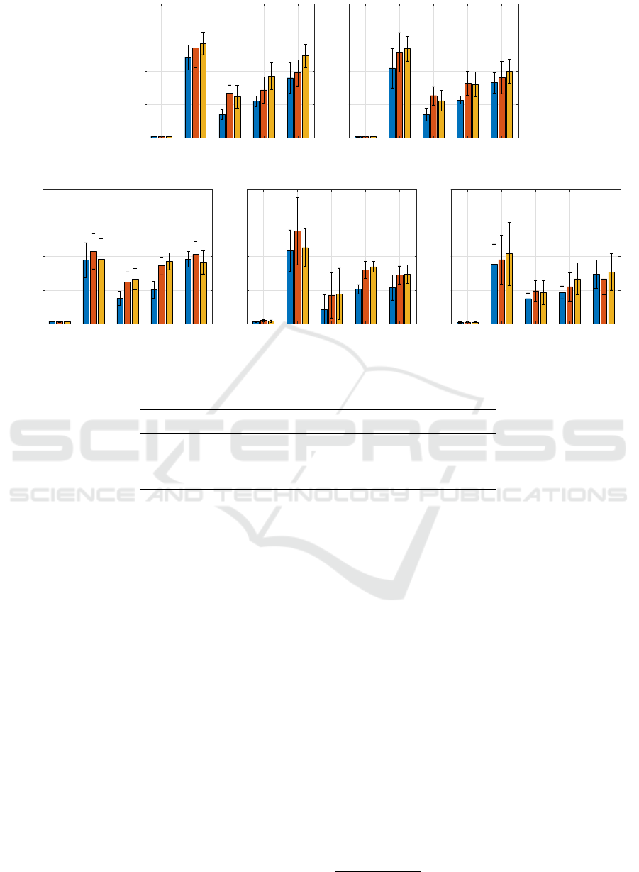
Figure 3: Selected number of symbols comparison for the 5 classiﬁers. For bar legend, see caption of Fig. 1.

Table 2: Average K value for K-NN classiﬁer, with standard deviation.

Sample % AIDS GREC Letter1 Letter2 Letter3

10 5 ± 4 3 ± 2 4 ± 4 1 ± 0 3 ± 3

30 8 ± 5 2 ± 1 5 ± 4 1 ± 0 4 ± 2

50 7 ± 4 2 ± 1 4 ± 4 1 ± 0 5 ± 5

ing between vertices is evaluated with a plain Eu-

clidean distance, whereas edge matching is a sim-

ple delta distance, being unlabelled.

GREC: patterns in this dataset are graph representa-

tion of symbols taken from architectural and elec-

tronic drawings. Since node labels are composed

by different data structures, a custom dissimilar-

ity measure is involved in the vertex matching, as

well as the edge dissimilarity function. In both

cases, dissimilarity measures are parametric with

respect to ﬁve real-valued parameters bounded in

[0, 1] whose values are stored in the set Π (cf. Eq.

(9)).

AIDS: graph instances in this dataset are molecular

compounds where atoms are represented as nodes

and covalent bonds as edges. Nodes dissimilarity

is a custom (non parametric) dissimilarity mea-

sure.

Further properties of these datasets and formal deﬁni-

tion of nodes and vertices dissimilarities can be found

in (Baldini et al., 2019b).

The software is developed in C++ using the

SPARE library (Livi et al., 2014). Additional depen-

dancies include LibSVM (Chang and Lin, 2011) for

ν-SVMs and the Boost Graph Library

for handling

graph data structures. In all tests, we adopt the Class-

Aware granulator (Baldini et al., 2019b) along with

the stochastic sampling method (Baldini et al., 2019a)

described in Section 3.2, where a Breadth First Search

strategy has been employed for graph traversing. In

this way, the cardinality of the set

L=1

g,tr

needed to

the granulator has been ﬁxed to a given number W as

percentage of the number of subraphs returned by the

exhaustive procedure (Bianchi et al., 2014a), reported

in Table 1. In order to take into account the intrinsic

randomness in the model synthesis procedure, we run

GRALG 10 times (both training and testing phases),

showing the results on the test set in terms of average

and standard deviation. For each of the ﬁve datasets,

training, validation and test splits are kept unchanged

with respect to the ones available in the IAM reposi-

tory.

The system parameters have been chosen as fol-

lows:

• W = 10%, 30%, 50% of the maximum number of

http://www.boost.org/

NCTA 2020 - 12th International Conference on Neural Computation Theory and Applications

346

subgraphs that can be drawn from the training set

(Table 1)

• Q ∈ [1, 500]

• o = 5 maximum subgraphs vertices

• 20 individuals per population of both genetic al-

gorithms

• 20 generations for the ﬁrst genetic algorithm (al-

phabet optimization)

• 50 generations for the second genetic algorithm

(feature selection)

• α = 0.99 in the ﬁtness function for the second ge-

netic algorithm (cf. Eq. (13))

• ε = 1.1 as tolerance value for the symbolic his-

tograms evaluation.

As the model complexity is concerned, we deﬁne R

as the ratio between complexity of the synthesized

model and its maximal attainable complexity:

• for SVMs, R reads as the ratio between the num-

ber of support vectors and |S

| (Martino et al.,

2020a);

• for ARC/PARC, one takes the ratio between the

number of hyperboxes and |S

| (Rizzi et al.,

2002);

• K-NN notably has the maximum complexity,

which equals |S

|, since all pairwise distances

with respect to the training data must be evalu-

ated for classiﬁcation. Notwithstanding that, for

the sake of completeness, we report the resulting

number of neighbours in Table 2.

In Fig. 1, we show the accuracy (both in terms

of average and standard deviation) obtained by the

ﬁve classiﬁers on the embedded version of the test

set S

, alongside the cardinality of the optimized al-

phabet A

∗

in Fig. 3. The latter simply reads as the

number of selected features after the second genetic

optimization and it can be considered as a measure

of model interpretability (the lower, the better). The

good performances obtained by ν-SVM are striking:

this classiﬁer outperforms the competitors especially

for GREC and Letter-H. On the other hand, its kernel-

ized counterpart shows generally poor performances

with respect to the rest of competitors. Notably, the

accuracy achieved on the three Letter datasets are

far from being comparable with the other methods.

This could be explained by considering that even if

a feature selection mechanism is employed, the re-

sulting embedding space is generally large, making

unnecessary or, as in this case, disadvantageous the

projection mapping due to kernel functions (Martino

et al., 2019a; Martino et al., 2020b). By observing

the number of selected features, the K-NN classiﬁer

emerges as the one that generally shows the smallest

number of symbols in the ﬁnal alphabet, especially

for Letter datasets, while keeping comparable perfor-

mances in terms of accuracy with the linear ν-SVM.

When we compare the classiﬁers in terms of struc-

tural complexity via the R score, as can be seen in

Fig. 2, Min-Max networks clearly show remarkable

behaviour with respect to SVMs. Indeed, even if ν-

SVMs have (slightly) better performances in terms

of accuracy, Min-Max networks strikingly outperform

them in terms of structural complexity. Further, it is

worth noting that RBF ν-SVMs in three cases (GREC,

Letter-M and Letter-H) tend to elect all patterns as

support vectors: a clear sign that they strive in dis-

criminating patterns in a Hilbert space.

5 CONCLUSIONS

In this paper, we proposed a comparison between dif-

ferent supervised learning algorithms for classifying

graphs in geometric spaces thanks to a graph embed-

ding procedure. Speciﬁcally, starting from GRALG,

whose embedding strategy relies on symbolic his-

tograms, we considered a ν-SVM equipped with lin-

ear and Gaussian kernels, a Min-Max neuro-fuzzy

network with two different training methods (namely,

ARC and PARC) and a simple K-NN decision rule.

The classiﬁers are evaluated by taking into account

both the accuracy on the test set and the R score for

the structural complexity. If on one hand these two

indices can summarize their classiﬁcation and gen-

eralization abilities, they do not consider the com-

plexity (dimensionality) of the underlying embedding

space. Consequently, the number of selected features

are considered as a futher performance measure of the

overall classiﬁcation system. At least for the con-

sidered datasets, our tests returned linear ν-SVM as

generally the most performing method and its kernel-

ized counterpart as the least performing one: this sug-

gests that non-linear kernels that implicitly map pat-

terns into higher dimensions may not work properly

with graph embedding strategies based on symbolic

histograms since the corresponding embedding vec-

tors are likely to reside in an already high dimensional

space. Notwithstanding their good performance, if

compared with ARC and PARC classiﬁers, SVMs

tend to have higher structural complexity. Under the

model interpretability viewpoint, K-NN seems to be

the most promising classiﬁer.

Complexity vs. Performance in Granular Embedding Spaces for Graph Classiﬁcation

347

REFERENCES

Bacciu, D., Micheli, A., and Sperduti, A. (2018). Gen-

erative kernels for tree-structured data. IEEE trans-

actions on neural networks and learning systems,

29(10):4932–4946.

Bai, L., Hancock, E. R., Han, L., and Ren, P. (2012). Graph

clustering using graph entropy complexity traces. In

Proceedings of the 21st International Conference on

Pattern Recognition (ICPR2012), pages 2881–2884.

Baldini, L., Martino, A., and Rizzi, A. (2019a). Stochastic

information granules extraction for graph embedding

and classiﬁcation. In Proceedings of the 11th Inter-

national Joint Conference on Computational Intelli-

gence - Volume 1: NCTA, (IJCCI 2019), pages 391–

402. INSTICC, SciTePress.

Baldini, L., Martino, A., and Rizzi, A. (2019b). Towards

a class-aware information granulation for graph em-

bedding and classiﬁcation. In Computational Intel-

ligence: 11th International Joint Conference, IJCCI

2019 Vienna, Austria, September 17-19, 2019 Revised

Selected Papers. To appear in.

Bargiela, A. and Pedrycz, W. (2003). Granular comput-

ing: an introduction. Kluwer Academic Publishers,

Boston.

Bargiela, A. and Pedrycz, W. (2006). The roots of granular

computing. In 2006 IEEE International Conference

on Granular Computing, pages 806–809.

Bianchi, F. M., Grattarola, D., Alippi, C., and Livi, L.

(2019). Graph neural networks with convolutional

arma ﬁlters. arXiv preprint arXiv:1901.01343.

Bianchi, F. M., Livi, L., Rizzi, A., and Sadeghian, A.

(2014a). A granular computing approach to the de-

sign of optimized graph classiﬁcation systems. Soft

Computing, 18(2):393–412.

Bianchi, F. M., Scardapane, S., Livi, L., Uncini, A., and

Rizzi, A. (2014b). An interpretable graph-based im-

age classiﬁer. In 2014 International Joint Conference

on Neural Networks (IJCNN), pages 2339–2346.

Bianchi, F. M., Scardapane, S., Rizzi, A., Uncini, A.,

and Sadeghian, A. (2016). Granular computing tech-

niques for classiﬁcation and semantic characterization

of structured data. Cognitive Computation, 8(3):442–

461.

Borgwardt, K. M. and Kriegel, H. P. (2005). Shortest-path

kernels on graphs. In Fifth IEEE International Con-

ference on Data Mining (ICDM’05), pages 8 pp.–.

Bunke, H. (2003). Graph-based tools for data mining and

machine learning. In Perner, P. and Rosenfeld, A., ed-

itors, Machine Learning and Data Mining in Pattern

Recognition, pages 7–19, Berlin, Heidelberg. Springer

Berlin Heidelberg.

Chang, C.-C. and Lin, C.-J. (2011). Libsvm: A library for

support vector machines. ACM transactions on intel-

ligent systems and technology (TIST), 2(3):27.

Cinti, A., Bianchi, F. M., Martino, A., and Rizzi, A. (2020).

A novel algorithm for online inexact string matching

and its fpga implementation. Cognitive Computation,

12(2):369–387.

Cover, T. and Hart, P. (1967). Nearest neighbor pattern clas-

siﬁcation. IEEE transactions on information theory,

13(1):21–27.

Ding, S., Du, M., and Zhu, H. (2015). Survey on granularity

clustering. Cognitive neurodynamics, 9(6):561–572.

Frattale Mascioli, F. M., Rizzi, A., Panella, M., and Mar-

tinelli, G. (2000). Scale-based approach to hierarchi-

cal fuzzy clustering. Signal Processing, 80(6):1001 –

1016.

Ghosh, S., Das, N., Gonçalves, T., Quaresma, P., and

Kundu, M. (2018). The journey of graph kernels

through two decades. Computer Science Review,

27:88 – 111.

Hamilton, W., Ying, Z., and Leskovec, J. (2017). In-

ductive representation learning on large graphs. In

Advances in neural information processing systems,

pages 1024–1034.

Han, L., Hancock, E. R., and Wilson, R. C. (2011). Charac-

terizing graphs using approximate von neumann en-

tropy. In Vitrià, J., Sanches, J. M., and Hernández,

M., editors, Pattern Recognition and Image Analysis,

pages 484–491, Berlin, Heidelberg. Springer Berlin

Heidelberg.

Kipf, T. N. and Welling, M. (2016). Semi-supervised clas-

siﬁcation with graph convolutional networks. arXiv

preprint arXiv:1609.02907.

Kondor, R. I. and Lafferty, J. (2002). Diffusion kernels on

graphs and other discrete structures. In Proceedings of

the 19th international conference on machine learn-

ing, volume 2002, pages 315–322.

Leone Sciabolazza, V. and Riccetti, L. (2020). Diffusion de-

lay centrality: Decelerating diffusion processes across

networks. Available at SSRN 3653030.

Levenshtein, V. I. (1966). Binary codes capable of correct-

ing deletions, insertions, and reversals. Soviet physics

doklady, 10(8):707–710.

Li, W. (2013). Modularity embedding. In Lee, M., Hirose,

A., Hou, Z.-G., and Kil, R. M., editors, Neural Infor-

mation Processing, pages 92–99, Berlin, Heidelberg.

Springer Berlin Heidelberg.

Livi, L., Del Vescovo, G., Rizzi, A., and Frattale Mascioli,

F. M. (2014). Building pattern recognition applica-

tions with the SPARE library. CoRR, abs/1410.5263.

Livi, L. and Rizzi, A. (2013). Graph ambiguity. Fuzzy Sets

and Systems, 221:24–47.

Martino, A., De Santis, E., Giuliani, A., and Rizzi, A.

(2020a). Modelling and recognition of protein contact

networks by multiple kernel learning and dissimilarity

representations. Entropy, 22(7).

Martino, A., Giuliani, A., and Rizzi, A. (2018a). Gran-

ular computing techniques for bioinformatics pat-

tern recognition problems in non-metric spaces. In

Pedrycz, W. and Chen, S.-M., editors, Computational

Intelligence for Pattern Recognition, pages 53–81.

Springer International Publishing, Cham.

Martino, A., Giuliani, A., and Rizzi, A. (2019a). (hy-

per)graph embedding and classiﬁcation via simplicial

complexes. Algorithms, 12(11).

Martino, A., Giuliani, A., Todde, V., Bizzarri, M., and

Rizzi, A. (2020b). Metabolic networks classiﬁcation

NCTA 2020 - 12th International Conference on Neural Computation Theory and Applications

348

and knowledge discovery by information granulation.

Computational Biology and Chemistry, 84:107187.

Martino, A., Rizzi, A., and Frattale Mascioli, F. M. (2018b).

Supervised approaches for protein function prediction

by topological data analysis. In 2018 International

Joint Conference on Neural Networks (IJCNN), pages

1–8.

Martino, A., Rizzi, A., and Frattale Mascioli, F. M.

(2019b). Efﬁcient approaches for solving the large-

scale k-medoids problem: Towards structured data.

In Sabourin, C., Merelo, J. J., Madani, K., and War-

wick, K., editors, Computational Intelligence: 9th In-

ternational Joint Conference, IJCCI 2017 Funchal-

Madeira, Portugal, November 1-3, 2017 Revised Se-

lected Papers, pages 199–219. Springer International

Publishing, Cham.

Mizui, Y., Kojima, T., Miyagi, S., and Sakai, O. (2017).

Graphical classiﬁcation in multi-centrality-index di-

agrams for complex chemical networks. Symmetry,

9(12).

Neumann, M., Garnett, R., Bauckhage, C., and Kersting,

K. (2016). Propagation kernels: efﬁcient graph ker-

nels from propagated information. Machine Learning,

102(2):209–245.

Niepert, M., Ahmed, M., and Kutzkov, K. (2016). Learning

convolutional neural networks for graphs. In Interna-

tional conference on machine learning, pages 2014–

2023.

Pedrycz, W. (2001). Granular computing: an introduction.

In Proceedings Joint 9th IFSA World Congress and

20th NAFIPS International Conference, volume 3,

pages 1349–1354. IEEE.

Pedrycz, W. (2005). Knowledge-based clustering: from

data to information granules. John Wiley & Sons.

Pedrycz, W. (2016). Granular computing: analysis and de-

sign of intelligent systems. CRC press.

Pedrycz, W. and Homenda, W. (2013). Building the

fundamentals of granular computing: A principle

of justiﬁable granularity. Applied Soft Computing,

13(10):4209 – 4218.

P˛ekalska, E. and Duin, R. P. (2005). The dissimilarity rep-

resentation for pattern recognition: foundations and

applications. World Scientiﬁc.

P˛ekalska, E., Duin, R. P., and Paclík, P. (2006). Prototype

selection for dissimilarity-based classiﬁers. Pattern

Recognition, 39(2):189–208.

Riesen, K. and Bunke, H. (2008). Iam graph database

repository for graph based pattern recognition and ma-

chine learning. In Joint IAPR International Work-

shops on Statistical Techniques in Pattern Recognition

(SPR) and Structural and Syntactic Pattern Recogni-

tion (SSPR), pages 287–297. Springer.

Rizzi, A., Del Vescovo, G., Livi, L., and Frattale Mascioli,

F. M. (2012). A new granular computing approach

for sequences representation and classiﬁcation. In The

2012 International Joint Conference on Neural Net-

works (IJCNN), pages 1–8.

Rizzi, A., Panella, M., and Frattale Mascioli, F. M. (2002).

Adaptive resolution min-max classiﬁers. IEEE Trans-

actions on Neural Networks, 13(2):402–414.

Schölkopf, B. and Smola, A. J. (2002). Learning with ker-

nels: support vector machines, regularization, opti-

mization, and beyond. MIT press.

Schölkopf, B., Smola, A. J., Williamson, R. C., and Bartlett,

P. L. (2000). New support vector algorithms. Neural

computation, 12(5):1207–1245.

Shawe-Taylor, J. and Cristianini, N. (2004). Kernel methods

for pattern analysis. Cambridge University Press.

Shervashidze, N. and Borgwardt, K. M. (2009). Fast subtree

kernels on graphs. In Advances in neural information

processing systems, pages 1660–1668.

Shervashidze, N., Schweitzer, P., Van Leeuwen, E. J.,

Mehlhorn, K., and Borgwardt, K. M. (2011).

Weisfeiler-lehman graph kernels. Journal of Machine

Learning Research, 12(9).

Shervashidze, N., Vishwanathan, S. V. N., Petri, T.,

Mehlhorn, K., and Borgwardt, K. M. (2009). Efﬁ-

cient graphlet kernels for large graph comparison. In

van Dyk, D. and Welling, M., editors, Proceedings of

the Twelfth International Conference on Artiﬁcial In-

telligence and Statistics, volume 5 of Proceedings of

Machine Learning Research, pages 488–495. PMLR.

Vishwanathan, S. V. N., Schraudolph, N. N., Kondor, R.,

and Borgwardt, K. M. (2010). Graph kernels. Journal

of Machine Learning Research, 11(Apr):1201–1242.

Wu, Z., Pan, S., Chen, F., Long, G., Zhang, C., and Philip,

S. Y. (2020). A comprehensive survey on graph neural

networks. IEEE Transactions on Neural Networks and

Learning Systems.

Xiao, B. and Hancock, E. R. (2005). Graph clustering using

heat content invariants. In Marques, J. S., Pérez de la

Blanca, N., and Pina, P., editors, Pattern Recognition

and Image Analysis, pages 123–130, Berlin, Heidel-

berg. Springer Berlin Heidelberg.

Xiao, B., Hancock, E. R., and Wilson, R. C. (2009). Graph

characteristics from the heat kernel trace. Pattern

Recognition, 42(11):2589–2606.

Ye, C., Wilson, R. C., and Hancock, E. R. (2014). Graph

characterization from entropy component analysis.

In 2014 22nd International Conference on Pattern

Recognition, pages 3845–3850.

Zadeh, L. A. (1979). Fuzzy sets and information granu-

larity. Advances in fuzzy set theory and applications,

11:3–18.

Zadeh, L. A. (1997). Toward a theory of fuzzy information

granulation and its centrality in human reasoning and

fuzzy logic. Fuzzy sets and systems, 90(2):111–127.

Zhang, S., Tong, H., Xu, J., and Maciejewski, R. (2019).

Graph convolutional networks: a comprehensive re-

view. Computational Social Networks, 6(1):11.

Complexity vs. Performance in Granular Embedding Spaces for Graph Classiﬁcation

349