XCSF for Automatic Test Case Prioritization

Lukas Rosenbauer

, Anthony Stein

, David P

atzel

and J

org H

ahner

BSH Home Appliances, Im Gewerbepark B35, Regensburg, Germany

Artiﬁcial Intelligence in Agricultural Engineering, University of Hohenheim, Garbenstr. 9, Stuttgart, Germany

Organic Computing Group, University of Augsburg, Eichleitnerstr. 30, Augsburg, Germany

joerg.haehner@informatik.uni-augsburg.de

Keywords:

Testing, Learning Classiﬁer Systems, Evolutionary Machine Learning, Reinforcement Learning.

Abstract:

Testing is a crucial part in the development of a new product. Due to the change from manual testing to

automated testing, companies can rely on a higher number of tests. There are certain cases such as smoke

tests where the execution of all tests is not feasible and a smaller test suite of critical test cases is necessary.

This prioritization problem has just gotten into the focus of reinforcement learning. A neural network and an

XCS classiﬁer system have been applied to this task. Another evolutionary machine learning approach is the

XCSF which produces, unlike XCS, continuous outputs. In this work we show that XCSF is superior to both

the neural network and XCS for this problem.

1 INTRODUCTION

Evolutionary computation has lead to several ad-

vances in testing. Rodrigues et al. (2018) examined

how a genetic algorithm (GA) can be used to gener-

ate test data. Nature inspired techniques have been ex-

ploited by Haga and Suehiro (2012) to automatically

generate test cases. Another application is to mutate

certain parts of the software to be tested in order to

detect how effective tests are (Jia and Harman, 2008).

The former has become its own ﬁeld called mutation

testing. Further GAs have been used to decide how

resources should be allocated in order to ensure how

reliability can be guaranteed (Dai et al., 2003).

Our use case is located in continuous integration

(CI) that is a practice in software development to fre-

quently integrate the work of each engineer. Thus

big forks that are hard to merge can be avoided and

software quality can be ensured. CI is made possible

by using an automation tool such as Jenkins (Smart,

2011). Jenkins can be used to checkout source code,

build it, test it, and deploy it. These steps are sum-

marized as pipelines (see Figure 1). One execution of

such a pipeline is called CI cycle.

checkout

source code

build

software

test

software

deploy

software

Figure 1: Example of a CI pipeline.

In this paper we concentrate solely on the testing

stage during which tests from any testing level may

run such as unit tests or even system tests. These

can vary in terms of their duration and ability to de-

tect failures. In some situations such as smoke test-

ing it is not feasible to run all tests as there is not

enough time (Dustin et al., 1999). Thus crucial tests

must be selected to form a test suite whose execu-

tion time does not exceed a given time budget. The

test suite should be adapted from cycle to cycle, re-

acting to code changes that inﬂuence the tests’ out-

comes. The desired test suite should be optimal in

terms of its ability to ﬁnd errors: Tests that can be

expected to pass should be skipped whereas tests that

would detect errors should be executed. Thus the tests

are to be ranked according to their ability to ﬁnd er-

rors. The prioritization and time budget induce the

test suite. The task of selecting such a prioritization

and test suite optimally is referred to as adaptive test

case selection problem (ATCS) (Spieker et al., 2017).

Spieker et al. (2017) and Rosenbauer et al. (2020)

exploit the fact that the CI infrastructure saves the

testing history (duration of tests, executions, test re-

sults). This information is used to construct a pri-

oritization of the test cases. During each CI cycle

the available test cases are parsed and ranked by re-

inforcement learning (RL) agents. An agent either

gets a penalty or a reward, based on the outcome

of the execution and the determined prioritization.

Rosenbauer, L., Stein, A., Pätzel, D. and Hähner, J.

XCSF for Automatic Test Case Prioritization.

DOI: 10.5220/0010105700490058

In Proceedings of the 12th International Joint Conference on Computational Intelligence (IJCCI 2020), pages 49-58

ISBN: 978-989-758-475-6

Spieker et al. (2017) employ a neural network-based

agent while Rosenbauer et al. (2020) utilize one based

on the XCS classiﬁer system (XCS) (Wilson, 1995).

XCS belongs to the family of learning classi-

ﬁer systems (LCS). LCSs are a framework of evo-

lutionary rule-based machine learning methods (Ur-

banowicz and Browne, 2017). Research for LCS goes

in multiple directions: mathematical examination as

documented by P

atzel et al. (2019), reduction of run-

time (Lanzi and Loiacono, 2010) or how the structure

of LCSs can be adapted to improve learning perfor-

mance (Stein et al., 2020). One such adaptation of

XCS is called XCSF. It differs from XCS as it has a

continuous output instead of a discrete one (Wilson,

2002). This is achieved by introducing polynomial

models as predictors to the classiﬁers of XCSF.

During this work we apply XCSF to the ATCS

problem. In order to do so, we examine three different

data sets. This has lead to the following contributions:

• We show that the piece-wise function approxima-

tion principle of XCSF is an advantage over XCS.

In all our experiments XCSF has an equal or bet-

ter performance.

• Rosenbauer et al. (2020) conducted a preliminary

study about the suitability of LCSs for ATCS. For

this they considered the three data sets and reward

functions that were used to benchmark the neu-

ral network of Spieker et al. (2017). The network

was in some cases superior to XCS. Our XCSF

approach is superior to the network in all but one

cases. If another reward function is used, then

XCSF is equal in terms of performance on this

data set.

We continue this paper with a brief discussion of

related work in Section 2. Afterwards we describe

ATCS in general and its interpretation as a RL prob-

lem. Further we describe the policy that we want to

use that is based on the approximation of a state-value

function (Section 3). In Section 4 we describe XCS

since XCSF is a mere extension of it. This is followed

by a description of how XCSF evolved from XCS and

how we adapted it for ATCS (Section 5). We bench-

mark our XCSF-based agent on three industrial data

sets against the neural network of Spieker et al. (2017)

and the XCS of Rosenbauer et al. (2020) in Section

6. We discuss possible future work in Section 7. We

close this work with a conclusion (Section 8).

2 RELATED WORK

Several approaches outside RL already exist to prior-

itize test cases. Di Nardo et al. (2015); Mirarab et al.

(2012) prioritize based on the coverage of the test

cases that requires a more detailed knowledge about

the underlying software. Gligoric et al. (2015) anal-

yse code dependencies to form a regression test suite.

Kwon et al. (2014) apply information retrieval tech-

niques to the source code and unit tests in order to

form a test suite. An entire survey about test case pri-

oritization was conducted by Marijan et al. (2013).

There are already several pure history-based ap-

proaches to form a prioritization (Park et al., 2008;

Jung-Min Kim and Porter, 2002; Noguchi et al.,

2015). The ﬁrst RL-based approach that solely relies

on historical data has been developed by Spieker et al.

(2017). Spieker et al. (2017) performed a competitive

study where they successfully compared their neural

network with several non-RL methods. The RL ap-

proach ensures easy integration into existing develop-

ment systems that enabled companies such as Netﬂix

to use it

. Rosenbauer et al. (2020) conducted a pre-

liminary study for the RL setting using XCS.

Epitropakis et al. (2015) developed a method to

ﬁnd a prioritization technique that intends to fulﬁll

several criteria. There are also several approaches

that are specialized for a speciﬁc form of testing such

as automotive (Haghighatkhah, 2020), user interfaces

(Nguyen et al., 2019) or production systems (Land

et al., 2019).

From a machine learning point of view our work

is deeply linked to LCS research. Applications range

from trafﬁc control (Tomforde et al., 2008), over dis-

tributed camera control (Stein et al., 2017) to manu-

facturing (Heider et al., 2020a). We are also not the

ﬁrst to apply XCSF to a real-world problem. It can

be used to control robots (Stalph et al., 2009) or for

image classiﬁcation (Lee et al., 2012). It is also worth

mentioning that XCSF is not the only LCS that pro-

vides a continuous output, for example SupRB’s ac-

tion space is also continuous (Heider et al., 2020b).

However, we are ﬁrst to our knowledge to apply

XCSF to a testing use case.

3 PROBLEM DESCRIPTION

In order to be consistent with the previous literature,

we follow the notation of Rosenbauer et al. (2020).

Let T be a test case. It has an estimated duration

of d(T ) and during CI cycle i there is a total execution

time of C available. During each CI cycle, each test

gets assigned a rank rk

(T ) which serves as a priority.

Ranks are not unique (it is possible for two tests to get

A corresponding article can be found here: Netﬂix

techblog

ECTA 2020 - 12th International Conference on Evolutionary Computation Theory and Applications

assigned the same rank). After this prioritization step,

a schedule is created that takes into account the time

budget available: The available tests are sorted de-

scendingly by their ranks, then, tests are taken repeat-

edly from the start of the resulting list until the sum

of the already selected tests’ estimated durations just

not yet exceeds the time budget. If there is not enough

time to schedule all tests of one rank, then tests of this

rank are selected uniformly at random until the termi-

nation criterion is met. Let l

(T ) be the index of a test

to bes executed T in the schedule. The selected tests

make up the test suite TS

which is executed as part of

CI cycle i. Let TS

be the test cases in TS

that failed

and TS

t,f

be the set of failed tests if all available tests

had been executed. The number of errors the test suite

found relative to TS

t,f

is then:

t,f

(1)

A widespread metric for evaluating the quality of a

test case prioritization is the normalized average per-

centage of faults detected (NAPFD) (Qu et al., 2007):

NAPFD(TS

) = p

−

∑

T ∈TS

(T )

|TS

| · |TS

2 · |TS

(2)

For NAPFD, high values are desired as small test

suites that detect many failures result in such high

values—especially if the failed tests were ranked

high. On the other hand, either failed tests with a

low rank or an increased number of high priority

tests which passed without error decrease the NAPFD

value. Thus, NAPFD measures the quality of both the

prioritization as well as the test suite.

Using the deﬁnition of NAPFD we are now able

to deﬁne the adaptive test case selection problem

(ATCS):

max NAPFD(TS

)

subject to

∑

T ∈TS

d(T) ≤ C

⊆ T

(3)

where T

denotes the set of available test during cycle

i. Thus the goal is the choice of TS

based on T

Similar to Spieker et al. (2017) and Rosenbauer

et al. (2020), we intend to solve ATCS using RL

which leads to the workﬂow described in Figure

2. The following paragraphs describe several possi-

ble reward functions as well as the state and action

spaces.

A reasonable thought is to try using the NAPFD

metric as a reward function for an agent. However, in

practice this would force us to always execute all tests

is needed for its computation) which we explicitly

want to avoid. Thus Spieker et al. (2017) came up

with three alternative reward functions. The ﬁrst is

the failure count reward

(T ) = |TS

| (4)

which does not distinguish between individual tests

as all receive the same reward. A more ﬁne-grained

approach is the test failure reward,

tcf

(T ) =

(

1 − v

(T ) T ∈ TS

0 otherwise,

(5)

where v

(T ) is the binary verdict of T during cycle

i with 0 indicating ‘test failed’ and 1 indicating ei-

ther of ‘test passed’ or ‘test not executed due to the

time restriction’. The advantage of r

tcf

over r

is that

it rewards tests individually based on their outcome.

However, it does not take the test’s rank into account

which has an impact on NAPFD. Thus Spieker et al.

(2017) came up with the time ranked reward

trk

(T ) = |TS

| − v

(T ) ·

∑

∈TS

rk(T )<rk(t

)

1 (6)

which still gives all failed test cases the same reward

but does distinguish the non-failed tests. These are

punished by the number of failed tests with a lower

rank. For example, a passed test that was correctly

ranked with a low priority will get a high reward and

a passed test with a high rank leads to a penalty. In

general, we denote the reward received at time t as

r(t).

The problem’s state space is deﬁned as follows:

S = [0,C] × {0, 1}

× [0, 1] (7)

The state (a test case) contains the approximated du-

ration (a real number between 0 and C), the testing

history (a binary vector of length k), and the time of

the last execution relative to the entire testing history

(a real number between 0 and 1). The hyperparam-

eter k indicates how many previous outcomes of the

test case are given to the agent. If there are not yet

k test results available, the missing entries are ﬁlled

with zeroes. States are vectors of dimension k+2; we

denote the state at time t by s(t).

The action space for both our XCSF-based solu-

tion as well as the network of Spieker et al. (2017) is

R whereas the XCS-based agent of Rosenbauer et al.

(2020) used an action space of {0, 1,. . ., 45}. We

write the action performed at time t as a(t).

It is worth mentioning that the RL interpretation

of ATCS slightly differs from the most common tem-

poral difference learning (TD) setting as, here, ﬁrst

all tests are ranked and only after the execution of the

tests of T

are rewards distributed. In TD, sequences

XCSF for Automatic Test Case Prioritization

test cases

agent

prioritized

test cases

selection &

scheduling

execution of

scheduled

tests

evaluation

rewards

Figure 2: Workﬂow for solving ATCS using RL.

of states, actions and rewards are usually observed un-

til a terminal state is observed:

s(1), a(1), r(1), s(2), a(2), r(2), . . . (8)

For ATCS, the sequence instead has the form

s(1), a(1), s(2), a(2). . . , s(n), a(n), r(1), r(2) . . . r(n)

(9)

with episodes corresponding to CI cycles (the termi-

nal state being the end of the cycle) which means

that the agent’s actions do not determine the length

of episodes. Also, the selection of states encountered

during an episode is ﬁxed as well as the test cases to

be ranked are known. However, it is worth mention-

ing that the environment may change from cycle to

cycle as new bugs may be introduced to the software

or existing ones may be ﬁxed (leading to additional

failed or succeeding tests, respectively).

A method often used for solving RL problems is

to approximate the state-action-value function (often

called Q-function) which assigns a measure of value

to each state-action pair (s, a) (e. g. the expected re-

turn when action a is performed in s and a certain

policy followed thereafter). Instead, our system ap-

proximates a state-value function V (·) for the follow-

ing policy π:

π(s) =

V(s) (10)

where

V(·) is the approximation of V (·). This pol-

icy follows a simple heuristic: A test case’s priority

should correspond to the value that can be achieved

or in other words if a test case (i. e. a state) has a high

value then it should have a high priority.

V(·) esti-

mates the reward that will be received if that policy is

applied. Thus our RL approach can also be seen as a

form of regression.

4 XCS CLASSIFIER SYSTEM

A learning classiﬁer system (LCS) roughly consists

of a population of rules, a learning mechanism for

them and an evolutionary heuristic to optimize their

localization in input space (usually a GA). The rules

are called classiﬁers and we denote one such rule by

cl. Each classiﬁer proposes an action cl.a to be ex-

ecuted if the conditions it speciﬁes are met by the

state s(t). Conditions can vary in their form depend-

ing on the problem. For example, a condition could

be a Boolean predicate that a value is in an interval.

Further, each classiﬁer tracks certain quality measures

that can be used to decide which rules of the popula-

tion should be applied.

A widespread LCS is the XCS classiﬁer system

(XCS) which was introduced by Wilson (1995). A

classiﬁer in XCS tracks how often it has been applied.

This is coined the classiﬁer’s experience. Further pa-

rameters include the classiﬁer’s predicted payoff cl.p

which estimates the return to be expected if the rule

is applied, an error estimate for that prediction cl.ε

and a niche-relative payoff prediction accuracy called

ﬁtness cl. f .

Whenever XCS classiﬁer system encounters a new

state s(t), it searches its population for classiﬁers

whose conditions are met (this is called matching).

If not enough classiﬁers are found then new ones are

created probabilistically whose conditions match s(t).

This process is called covering. The found and newly

created classiﬁers make up the match set M

. Based

on the match set XCS computes a quality measure

called system prediction, the ﬁtness-weighted sum of

predicted payoffs, for each action in available in the

match set:

∑

cl∈M

,cl.a=a

cl.p · cl. f

∑

cl∈M

,cl.a=a

cl. f

(11)

These values make up the prediction array PA

which

is used as a base for decision-making. XCS usually

either chooses the action at random to explore the en-

vironment or according to the highest system predic-

tion value. After it has decided for an action it selects

all classiﬁers of M

that propose the chosen action and

summarizes them in the action set A

. After the exe-

cution of the chosen action, XCS receives a reward

which is used to calculate the update target P:

P = r(t) + γ · max(PA

t+1

) (12)

ECTA 2020 - 12th International Conference on Evolutionary Computation Theory and Applications

where γ is the usual reinforcement learning discount-

ing factor. It is used to update the classiﬁers of

the previous action set A

t−1

such that each classiﬁer

learns to model the expected return received when its

action is executed for states that match its conditions.

XCS additionally employs a genetic algorithm to

optimize the conditions of the classiﬁers available. Its

task is to ﬁnd an optimal partition of the classiﬁers

for the problem surface by adapting their localization.

The heuristic creates new classiﬁers based on existing

ones of the population by applying crossover and mu-

tation operators on their conditions. The GA is used

periodically (e. g. after every tenth state encountered).

The population of XCS has a ﬁxed capacity. After

each execution of the GA and the matching process,

its size is checked. If the population has too many ele-

ments then XCS deletes classiﬁers at random but pro-

portional to their quality. We call this deletion mech-

anism pruning.

We describe the basic workﬂow of XCS in Al-

gorithm 1. The function choose action employs a ε-

greedy policy to select the next action (Butz and Wil-

son, 2001). We keep the description of XCS at this

abstract level but recommend to read Urbanowicz and

Browne (2017) where LCSs are described in detail.

Algorithm 1: XCS workﬂow based on Butz and

Wilson (2001).

input : s(t), r(t − 1)

1 M

= matching(population, s(t))

2 PA

= prediction array(M

)

3 a = choose action(PA

)

4 A

= get action set(M

, a)

5 execute a, observe r(t)

6 P = r(t − 1) + γ max(PA

)

7 // if non-empty

8 update A

t−1

by P

9 A

t−1

= A

10 if GA should run then

11 run GA on A

12 prune population

Rosenbauer et al. (2020) adapted XCS to the prob-

lem as it originally follows the usual TD learning

scheme based on the sequence of states, actions and

rewards given in Equation 8 and not the sequence

given in Equation 9. In order to adapt XCS to the

problem they introduced a batch update rule. Instead

of using the maximum system prediction of the suc-

ceeding state, they use the average maximum system

prediction of the states of the succeeding CI cycle to

compute P:

P = r(t) + γ ·

∑

j∈e

i+1

max(PA

)

i+1

(13)

where e

i+1

denotes the time steps of the cycle i + 1.

Further, the classiﬁers are always updated at the end

of a cycle and not between two states. In our later

experiments we simply call this variant XCS.

Additionally, Rosenbauer et al. (2020) examined

whether a experience replay version of XCS can im-

prove results for ATCS. However, this proved to be

detrimental in most cases which is why we do not in-

clude that version in our later experiments.

5 FROM XCS TO XCSF

XCS as proposed by Wilson (1995) produces a dis-

crete output (the actions). Some problems, however,

have a more continuous nature. Thus Wilson (2002)

adapted XCS to also provide a real-valued output

which resulted in the XCSF classiﬁer system, a gen-

eral function approximator. In our use case we use

XCSF to approximate V (·) as already mentioned in

Section 3 which enables us to use continuous actions.

In contrast to standard XCS, a classiﬁer in XCSF

does not have a scalar prediction. Instead its predic-

tion is modelled as a function that approximates the

expected payoff. Here we model the classiﬁer’s pre-

diction function as follows:

cl. p(s) = w

k+2

∑

i=1

· s

(14)

where s is an element of the state space and w

repre-

sent real-valued weights. Initially the weights are set

randomly. The weights are updated using a gradient-

descent-based method called modiﬁed delta rule (Wil-

son, 2002):

∆w

k ˜sk

(r − cl.p(s))˜s

(15)

The old estimation of w

is simply updated by adding

∆w

. Here η denotes the learning rate which controls

how strongly a new experience can inﬂuence the cur-

rent estimator. The vector ˜s is the same as the state

vector s but with an additional of 1 for ﬁtting the in-

tercept:

˜s = (1, s

, s

, ..., s

k+2

)

(16)

Further, k ˜sk is the euclidean norm of ˜s and r is the

reward that corresponds to the state s. Thus we do

not use P of Equation 12 as an update target, but the

actual reward.

XCSF classiﬁers only maintain a dummy action

(in order to stick to the original workﬂow of XCS).

Hence XCSF computes only one system prediction as

follows:

∑

cl∈M

cl.p(s(t)) · cl. f

∑

cl∈M

cl. f

(17)

XCSF for Automatic Test Case Prioritization

which is used as estimation for the function to be ap-

proximated (in our case V (s(t))). We directly use the

estimation as action as we employ the policy of Equa-

tion 10.

For XCSF, the match set is equal to the action set.

Hence all matching classiﬁers are updated whenever

a reward is received. Further M

is updated using r(t).

In our experiments we employ a batch update

mode as we only receive rewards at the end of a CI

cycle. Thus during the prioritization of tests we solely

choose ranks and save the action sets that will be up-

dated as described in Algorithm 2. At the end of the

cycle we update the collected action sets, run the GA

and prune the population (see Algorithm 3).

It is worth mentioning that we further differ from

Wilson (2002) as the states s also contain binary vari-

ables instead of exclusively real numbers. We can still

ﬁt our linear models cl.p(·) since gradient-descent

based methods such as the modiﬁed delta rule only

require continuous weights and not continuous states

(as the weights are optimized) (Aggarwal, 2020).

Algorithm 2: Action selection of XCSF.

input : state s

output: action a

1 M

= matching(population, s)

2 a =

∑

cl∈M

cl.p(s)·cl. f

∑

cl∈M

cl. f

3 A

= M

4 cycle action sets.append(A

)

5 return a

Algorithm 3: XCSF batch update learning.

input: rewards of CI cycle

1 for j = 1 to length(rewards) do

2 update cycle action sets[j] by rewards[j]

3 if GA should run then

4 run GA on cycle action sets[j]

5 end

6 cycle action sets = {}

7 prune population

6 EVALUATION

In our experiments we compare our batch update

XCSF with the XCS variant of Rosenbauer et al.

(2020) and the artiﬁcial neural network approach of

Spieker et al. (2017). We reuse the three data sets of

Spieker et al. (2017). The ﬁrst two are from a Scan-

dinavian robot company and called ABB paint control

and ABB IOF/ROL. Additionally the Google shared

data set of test suite results (GSDTSR) is considered.

2 3 4 5 6 7 8

History Length

100

% of best result

XCS

XCSF

Network

Figure 3: Evaluation of the history length’s inﬂuence on

performance. The y-axis displays the average NAPFD val-

ues of the methods in relation to the best average NAPFD

achieved.

Table 1: Examined data sets.

paint IOF/ROL GSDTSR

control

CI cycles 312 320 336

test cases 114 2,086 5,555

verdicts 25,594 30,319 1,260,617

failed 19.36% 28.43% 0.25%

Table 1 gives a brief overview about the structure of

these data sets. All three data sets vary in terms of

their test cases, verdicts, and amount of failed tests.

Thus we can examine the three methods on a broader

scope.

Table 2: P-Values for paired Student t-tests (rounded to the

ﬁfth decimal). Values below 0.05 are marked bold. The null

hypothesis is that XCS is superior to XCSF.

Paint Control IOF/ROL GSDTSR

0.00523 0.25042 0.0002

tcf

0.30446 0.32404 0.00091

trk

0.00192 0.14235 0.00001

Table 3: P-Values for paired Student t-tests (rounded to the

ﬁfth decimal). Values below 0.05 are marked bold. The null

hypothesis is that the neural network is superior to XCSF.

Paint Control IOF/ROL GSDTSR

0.0 0.01473 0.0

tcf

0.99999 0.00015 0.0

trk

0.0 0.00078 0.0

For the XCS-based agent and the neural network

we can rely on the original implementation. Both

were also benchmarked on the same data sets that

we consider. We adopted the original hyperparame-

ters proposed by Spieker et al. (2017) and Rosenbauer

et al. (2020) for each respective agent, respectively.

This way, we ensure a fair comparison with our ap-

proach.

ECTA 2020 - 12th International Conference on Evolutionary Computation Theory and Applications

0.00

0.25

0.50

0.75

1.00

NAPFD

ABB Paint Control

Network

XCS

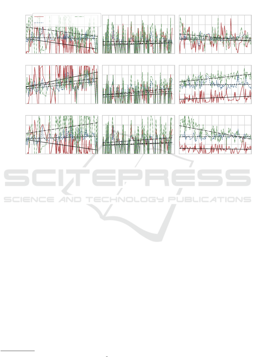
XCSF

ABB IOF/ROL

(a) Failure Count Reward

GSDTSR

0.00

0.25

0.50

0.75

1.00

NAPFD

(b) Test Case Failure Reward

60 120 180 240 300

CI Cycle

0.00

0.25

0.50

0.75

1.00

NAPFD

60 120 180 240 300

CI Cycle

0 60 120 180 240 300

CI Cycle

Figure 4: Comparison of XCSF with XCS and the neural network.

To our knowledge there is no XCSF library for

states that both have binary and real valued compo-

nents. Hence we had to implement our own XCSF

which we did in Python 3

. We modelled the condi-

tions for the real values as intervals and for the binary

parts of the states we follow the original XCS and use

ternary conditions (Wilson, 1995). For the GA we use

a roulette wheel selection-based on the classiﬁer’s ﬁt-

ness. For the crossover of the ternary conditions we

apply a one-point crossover and for the intervals and

weights of cl.p(·) an arithmetic one. For the muta-

tion of the ternary conditions we follow Butz and Wil-

son (2001) and for the interval-based conditions and

weights of cl.p(·) we apply a random mutation (i. e.

choosing an entirely random interval). We don’t per-

form any form of subsumption.

We set the learning rate η to 0.1. We draw the ini-

tial weights of cl.p(·) during covering and mutation

uniform at random from [−10,10]. For the remaining

hyperparameters we follow the notation of Butz and

Wilson (2001). The population capacity N is 2000. α

and β are set to 0.15, ν is 5, θ

is 25, µ is 0.025. The

initial error ε

and initial ﬁtness f

of the classiﬁers is

set to 0. θ

del

is 20, θ

sub

is 20, χ is 0.75, p

exp

is 0.2 and

source code: https://github.com/LagLukas/xcsf atcs

is 0.01. During covering we set a binary condition

to # with a probability of 0.33.

We perform thirty i.i.d. runs for every experiment

and display the averaged results. We can simulate the

real use case as we have the results of all test cases for

every CI cycle. Thus we can use the reward functions

of Section 3 whilst being able to evaluate the perfor-

mance of the methods in terms of NAPFD.

In our ﬁrst experiment we evaluate the inﬂuence

of the history length k on the performance. We ex-

amine the lengths k = 2, 3, .., 8. For all methods we

use the time ranked reward function. The results can

be seen in Figure 3. The x-axis shows the values for

k and the y-axis shows the average NAPFD values of

the methods relative to the best. XCSF clearly ex-

ceeds the two RL agents for this combination of re-

ward function and data set. We veriﬁed this visual

observation with a series of one-sided paired Student-

t tests which were signiﬁcant. We further veriﬁed the

necessary condition of normal distributed data with

Shapiro-Wilk tests. For these tests we used a signiﬁ-

cance level of 0.05.

Furthermore we could observe that a higher value

of k is beneﬁcial for XCSF. Thus we will use a his-

tory length of 8 in the upcoming experiments. For the

other agents the history length does not seem to affect

XCSF for Automatic Test Case Prioritization

their performance too much. However, this is only

one out of nine possible combinations of reward func-

tion and data set. Hence we consider now all three

data sets and reward functions in order to examine the

performance of XCSF on a wider scope.

The results are displayed in Figure 4. Each col-

umn contains the results for one data set and each row

represents the experimental outcome for one reward

function. Each plot contains a trendline for every ex-

amined agent next to the averaged results.

We provide additional statistical tests in Table 2

and 3 as we deem a purely visual evaluation as insufﬁ-

cient. Especially as trendlines can easily be disturbed

by statistical outliers. The tables contain p-values of

paired Student-t tests where we marked p-values be-

low 0.05 as signiﬁcant. The necessary condition of

normal distributed data was conﬁrmed by Shapiro-

Wilk tests (using a signiﬁcance level of 0.05).

On the paint control data set (column 1) we can

see that XCSF is superior to XCS (in terms of the

trendline) for all reward functions but the perfor-

mance, if the failure count reward is used, seems

to decline over time. Statistical tests can conﬁrm

XCSF’s superiority for the failure count reward and

the time ranked reward. For the test case failure re-

ward the p-value is not signiﬁcant and thus we per-

formed an additional t-test to test the nullhypothesis

that XCSF is superior to XCS. The latter test was also

not signiﬁcant and thus we deem both systems equiv-

alent for this combination of data set and reward func-

tion. However, we can observe the best performance

for XCSF for the time ranked reward and there it

clearly exceeds XCS regardless of the reward function

in terms of NAPFD. XCSF is also able to outperform

the neural network in two out of three cases. Visu-

ally we cannot determine if XCSF combined with the

time ranked reward or the network combined with the

test case failure reward is better suited for this data set

or vice versa. Additional paired Student-t tests could

also not reveal which approach is superior. Hence we

deem both methods as equivalent for this problem.

For the IOF/ROL data (column 2) the trendlines

indicate that XCSF is superior to XCS but statistical

tests cannot conﬁrm this observation (see Table 2).

We additionally tested the nullhypothses that XCSF

is superior to XCS and we could also not reject these.

Hence we deem XCS and XCSF equivalent on this

data set. On the other hand the statistical evaluation

shows that XCSF is superior to the neural network.

However, all three approaches have difﬁculties learn-

ing a good policy on this data set as the NAPFD re-

sults are generally worse than on the paint control data

set.

Column 3 displays the results for the GSDTSR

data set. For the failure count reward and the time

ranked reward the performance of XCSF seems to de-

cline over time and ﬁnally falls behind XCS. Due to

the high NAPFD values for most CI cycles the statis-

tical tests state that XCSF is better. However, visu-

ally the best approach for this data set is XCSF com-

bined with the test case failure reward. This com-

bination does not only outperform the XCS but also

the neural network for all three reward functions (in

terms of NAPFD). Furthermore it is also the only set-

ting where we can observe a positive slope for the

trendline. Spieker et al. (2017) and Rosenbauer et al.

(2020) deemed this as rather unlikely to achieve as the

data set contains very few failed tests.

We also observed that the structure of the data set

should also be considered for the choice of the reward

function for XCSF (Hamid and Braun, 2019). If the

data set contains very few failed tests then the time

ranked reward function proofs detrimental (see GS-

DTSR) but if it contains a certain amount of failures

then it seems to be a good choice (see ABB data sets).

7 FUTURE WORK

We further want to boost the results of XCSF by using

interpolation (Stein et al., 2018; Stein et al., 2016).

The application of interpolation to certain parts of

XCSF such as the GA can improve learning efﬁ-

ciency.

Another new direction in machine learning is to

generate new experiences from previous ones (also by

applying interpolation) and use them for training. von

Pilchau et al. (2020) showed in a preliminary study

that this proofs useful for artiﬁcial neural networks.

The same could be the case for LCSs such as XCSF.

Further, we only applied linear functions for the

classiﬁers. Lanzi et al. (2005) showed that polyno-

mial functions of higher order such as cubic ones can

also be beneﬁcial for XCSF.

Furthermore we think that the performance of

XCSF can be improved by using more information

such as changelogs, git diffs or additional test meta-

data.

8 CONCLUSION

During this work we evaluated the test case priori-

tization problem coined adaptive test case selection

problem (ATCS). Recently it has been interpreted as

reinforcement learning problem and two agents are

known in literature; an XCS-based one (Rosenbauer

ECTA 2020 - 12th International Conference on Evolutionary Computation Theory and Applications

et al., 2020) and an approach using an artiﬁcial neural

network-based (Spieker et al., 2017).

We used a XCSF-based agent and employed a

simple heuristic: a test case of high value should have

a high priority. Hence we used XCSF to approximate

a state-value function V (·) and interpreted the approx-

imated values as actions.

We benchmarked our agent on three different data

sets using three reward functions. In our comparison,

XCSF was in 8 out of 9 cases superior to the neural

network. For a single combination of reward func-

tion and data set XCSF was inferior. However, if the

best combinations of reward functions and agent are

considered on the data set then both approaches are

equal.

Our experiments showed that the continuous out-

put leads to a performance boost compared to XCS as

XCSF was in all nine cases considered either superior

or had an equivalent performance. Thus we recom-

mend to use XCSF for ATCS.

REFERENCES

Aggarwal, C. (2020). Linear Algebra and Optimization for

Machine Learning: A Textbook.

Butz, M. V. and Wilson, S. W. (2001). ”An Algorithmic

Description of XCS”. In Luca Lanzi, P., Stolzmann,

W., and Wilson, S. W., editors, Advances in Learn-

ing Classiﬁer Systems, pages 253–272, Berlin, Hei-

delberg. Springer Berlin Heidelberg.

Dai, Y., Xie, M., Poh, K., and Yang, B. (2003). ”Optimal

testing-resource allocation with genetic algorithm for

modular software systems”. Journal of Systems and

Software, 66(1):47 – 55.

Di Nardo, D., Alshahwan, N., Briand, L., and Labiche, Y.

(2015). Coverage-based regression test case selection,

minimization and prioritization: a case study on an

industrial system. Software Testing, Veriﬁcation and

Reliability, 25(4):371–396.

Dustin, E., Rashka, J., and Paul, J. (1999). Automated Soft-

ware Testing: Introduction, Management, and Perfor-

mance. Addison-Wesley Longman Publishing Co.,

Inc., USA.

Epitropakis, M. G., Yoo, S., Harman, M., and Burke, E. K.

(2015). Empirical evaluation of pareto efﬁcient multi-

objective regression test case prioritisation. In ISSTA

2015.

Gligoric, M., Eloussi, L., and Marinov, D. (2015). Ekstazi:

Lightweight Test Selection. In 2015 IEEE/ACM 37th

IEEE International Conference on Software Engineer-

ing, volume 2, pages 713–716.

Haga, H. and Suehiro, A. (2012). Automatic test case gen-

eration based on genetic algorithm and mutation anal-

ysis. In 2012 IEEE International Conference on Con-

trol System, Computing and Engineering, pages 119–

123.

Haghighatkhah, A. (2020). Test case prioritization using

build history and test distances: an approach for im-

proving automotive regression testing in continuous

integration environments.

Hamid, O. H. and Braun, J. (2019). Reinforcement Learn-

ing and Attractor Neural Network Models of Associa-

tive Learning, pages 327–349. Springer International

Publishing, Cham.

Heider, M., P

atzel, D., and H

ahner, J. (2020a). Towards

a Pittsburgh-Style LCS for Learning Manufacturing

Machinery Parametrizations. In Proceedings of the

2020 Genetic and Evolutionary Computation Confer-

ence Companion, GECCO ’20, page 127–128, New

York, NY, USA. Association for Computing Machin-

ery.

Heider, M., P

atzel, D., and H

ahner, J. (2020b). SupRB: A

Supervised Rule-based Learning System for Continu-

ous Problems.

Jia, Y. and Harman, M. (2008). Constructing Subtle Faults

Using Higher Order Mutation Testing. In 2008 Eighth

IEEE International Working Conference on Source

Code Analysis and Manipulation, pages 249 – 258.

Jung-Min Kim and Porter, A. (2002). A history-based test

prioritization technique for regression testing in re-

source constrained environments. In Proceedings of

the 24th International Conference on Software Engi-

neering. ICSE 2002, pages 119–129.

Kwon, J., Ko, I., Rothermel, G., and Staats, M. (2014). Test

Case Prioritization Based on Information Retrieval

Concepts. In 2014 21st Asia-Paciﬁc Software Engi-

neering Conference, volume 1, pages 19–26.

Land, K., Cha, S., and Vogel-Heuser, B. (2019). An

Approach to Efﬁcient Test Scheduling for Auto-

mated Production Systems. 2019 IEEE 17th Interna-

tional Conference on Industrial Informatics (INDIN),

1:449–454.

Lanzi, P. L. and Loiacono, D. (2010). ”Speeding Up Match-

ing in Learning Classiﬁer Systems Using CUDA”. In

Bacardit, J., Browne, W., Drugowitsch, J., Bernad

Mansilla, E., and Butz, M. V., editors, Learning

Classiﬁer Systems, pages 1–20, Berlin, Heidelberg.

Springer Berlin Heidelberg.

Lanzi, P. L., Loiacono, D., Wilson, S. W., and Goldberg,

D. E. (2005). Extending xcsf beyond linear approxi-

mation. In Proceedings of the 7th Annual Conference

on Genetic and Evolutionary Computation, GECCO

’05, page 1827–1834, New York, NY, USA. Associa-

tion for Computing Machinery.

Lee, P., Teng, Y., and Hsiao, T.-C. (2012). XCSF for Predic-

tion on Emotion Induced by Image Based on Dimen-

sional Theory of Emotion. In Proceedings of the 14th

Annual Conference Companion on Genetic and Evo-

lutionary Computation, GECCO ’12, page 375–382,

New York, NY, USA. Association for Computing Ma-

chinery.

Marijan, D., Gotlieb, A., and Sen, S. (2013). Test Case Pri-

oritization for Continuous Regression Testing: An In-

dustrial Case Study. In 2013 IEEE International Con-

ference on Software Maintenance, pages 540–543.

Mirarab, S., Akhlaghi, S., and Tahvildari, L. (2012). Size-

Constrained Regression Test Case Selection Using

XCSF for Automatic Test Case Prioritization

Multicriteria Optimization. IEEE Transactions on

Software Engineering, 38(4):936–956.

Nguyen, A., Le, B., and Nguyen, V. (2019). Prioritizing

Automated User Interface Tests Using Reinforcement

Learning. In Proceedings of the Fifteenth Interna-

tional Conference on Predictive Models and Data An-

alytics in Software Engineering, PROMISE’19, page

56–65, New York, NY, USA. Association for Comput-

ing Machinery.

Noguchi, T., Washizaki, H., Fukazawa, Y., Sato, A., and

Ota, K. (2015). History-Based Test Case Prioritization

for Black Box Testing Using Ant Colony Optimiza-

tion. In 2015 IEEE 8th International Conference on

Software Testing, Veriﬁcation and Validation (ICST),

pages 1–2.

Park, H., Ryu, H., and Baik, J. (2008). Historical Value-

Based Approach for Cost-Cognizant Test Case Prior-

itization to Improve the Effectiveness of Regression

Testing. In 2008 Second International Conference

on Secure System Integration and Reliability Improve-

ment, pages 39–46.

atzel, D., Stein, A., and H

ahner, J. (2019). A Survey

of Formal Theoretical Advances Regarding XCS. In

Proceedings of the Genetic and Evolutionary Com-

putation Conference Companion, GECCO ’19, pages

1295–1302, New York, NY, USA. ACM.

Qu, X., Cohen, M. B., and Woolf, K. M. (2007). Com-

binatorial Interaction Regression Testing: A Study of

Test Case Generation and Prioritization. In 2007 IEEE

International Conference on Software Maintenance,

pages 255–264.

Rodrigues, D. S., Delamaro, M. E., Corr

ea, C. G., and

Nunes, F. L. S. (2018). Using Genetic Algorithms in

Test Data Generation: A Critical Systematic Mapping.

ACM Comput. Surv., 51(2).

Rosenbauer, L., Stein, A., Maier, R., P

atzel, D., and H

ahner,

J. (2020). XCS as a Reinforcement Learning Ap-

proach to Automatic Test Case Prioritization. In Pro-

ceedings of the Genetic and Evolutionary Computa-

tion Conference Companion, GECCO ’20.

Smart, J. F. (2011). Jenkins: The Deﬁnitive Guide. O’Reilly,

Beijing.

Spieker, H., Gotlieb, A., Marijan, D., and Mossige, M.

(2017). Reinforcement Learning for Automatic Test

Case Prioritization and Selection in Continuous Inte-

gration. In Proceedings of the 26th ACM SIGSOFT In-

ternational Symposium on Software Testing and Anal-

ysis, ISSTA 2017, page 12–22, New York, NY, USA.

Association for Computing Machinery.

Stalph, P. O., Butz, M. V., and Pedersen, G. K. M. (2009).

Controlling a Four Degree of Freedom Arm in 3D

Using the XCSF Learning Classiﬁer System. In

Mertsching, B., Hund, M., and Aziz, Z., editors, KI

2009: Advances in Artiﬁcial Intelligence, pages 193–

200, Berlin, Heidelberg. Springer Berlin Heidelberg.

Stein, A., Eym

uller, C., Rauh, D., Tomforde, S., and

ahner, J. (2016). Interpolation-based classiﬁer gen-

eration in XCSF. In 2016 IEEE Congress on Evolu-

tionary Computation (CEC), pages 3990–3998.

Stein, A., Maier, R., Rosenbauer, L., and H

ahner, J. (2020).

XCS Classiﬁer System with Experience Replay. In

Proceedings of the Genetic and Evolutionary Compu-

tation Conference Companion, GECCO ’20.

Stein, A., Menssen, S., and H

ahner, J. (2018). What about

Interpolation? A Radial Basis Function Approach to

Classiﬁer Prediction Modeling in XCSF. In Proceed-

ings of the Genetic and Evolutionary Computation

Conference, GECCO ’18, page 537–544, New York,

NY, USA. Association for Computing Machinery.

Stein, A., Rudolph, S., Tomforde, S., and H

ahner, J. (2017).

Self-Learning Smart Cameras – Harnessing the Gen-

eralization Capability of XCS.

Tomforde, S., Prothmann, H., Rochner, F., Branke, J.,

ahner, J., M

uller-Schloer, C., and Schmeck, H.

(2008). Decentralised Progressive Signal Systems for

Organic Trafﬁc Control. pages 413–422.

Urbanowicz, R. J. and Browne, W. N. (2017). Introduction

to Learning Classiﬁer Systems. Springer Publishing

Company, Incorporated, 1st edition.

von Pilchau, W. P., Stein, A., and H

ahner, J. (2020). Boot-

strapping a DQN Replay Memory with Synthetic Ex-

periences. ArXiv, abs/2002.01370.

Wilson, S. (2002). Classiﬁers that Approximate Functions.

Natural Computing, 1:1–2.

Wilson, S. W. (1995). Classiﬁer Fitness Based on Accuracy.

Evolutionary Computation, 3(2):149–175.

ECTA 2020 - 12th International Conference on Evolutionary Computation Theory and Applications