Dynamic Error Compensation Model of Articulated Arm Coordinate

Measuring Machine

Jiaqi Zhu

1, a

, Xugang Feng

1, b, *

and Jiayan Zhang

1, c

School of Electrical and Information Engineering, Anhui University of Technology, Ma’anshan 243032, China

Keywords: Neural network, Simulated annealing algorithm, Flexible arm coordinate measuring machine, Error

compensation.

Abstract: The error factors of articulated arm coordinate measuring machine (AACMM) are many and the

relationship between them is nonlinear, which is difficult to establish the model by traditional mathematical

modeling. This paper analyses the error sources, on the basis of parameter calibration, to select the angle

coding, thermal deformation and probe system as the research object and introduce coordinate values to

indirectly describe the remaining errors in the model. The BP neural network is used to build up the error

compensation model, connection weights of the neural network are optimized by the modified simulated

annealing (MSA) algorithm, which solves the problem that the neural network is easy to fall into the local

minimum and the susceptible to interference. The data samples are obtained through experiments, and the

test data are utilized to exercise model built. The experimental result demonstrates that the average value of

the single point repeatability error after compensation is reduced from 0.1782 mm to 0.0383 mm.

1 INTRODUCTION

The articulated arm coordinate measuring machine

(AACMM) generally having 6 degrees of freedom is

a non-orthogonal coordinate system measuring

device that simulates the structure of the human arm.

It has broad application prospects, not only can

complete online measurement and evaluation on the

assembly line, but also suitable for outdoor

measurement and occasions where the object tested

is inconvenient to move. The advantages involves of

easy portability, low price, flexible measurement,

large measuring range and practicality in the field.

Due to its series-space open-chain structure, the

measurement error has the characteristics of

accumulation, transmission and amplification during

the measurement process, ultimately leading to poor

overall performance of the measuring machine (Zhao

H N, Yu L D, Jia H K, et al, 2016; Feng X G, Xu C,

Zhang J Y, et al, 2016; Fedorov V G, 2008; Romdhani F ,

François Hennebelle, Ge M , et al, 2015; Xing H L, Bo C,

Zu R Q, 2013).

At present, the AACMM mainly reduces the

error by calibrating the structural parameters

according to calibration algorithm or external high-

precision equipment. For example, Santolaria J et al

established an error model based on Fourier

polynomial and estimated the parameter error of the

AACMM machine by using a spherical gauge with

14 spheres (SANTOLARIA J., AGUILAR J.J. YAGUE

J.A., et al, 2008). ACERO studied the feasibility of

laser tracker as a reference instrument in AACMM

parameter calibration (ACERO R., BRAU A.,

SANTOLARIA J., et al, 2015). Zheng D T established

the spatial point error model and spatial error

distribution of the AACMM by using the basic

theory of functional network and the principle of

vector machine (Zheng D T, FEI Y T, 2010).

However, there are many error factors in the

AACMM, and the structural parameters are only a

part of it. This paper analyzes the error sources in

the measurement space and applies a method based

on the improved simulated annealing algorithm to

optimize the neural network to model the multiply

error of the coordinate measuring machine. By

comparing the results, the validity of the

compensation model is verified.

2 ERROR ANALYSIS

The AACMM is composed of three joint arms and

one probe combined through six rotary joints in

210

Zhu, J., Feng, X. and Zhang, J.

Dynamic Error Compensation Model of Articulated Arm Coordinate Measuring Machine.

DOI: 10.5220/0008856502100216

In Proceedings of 5th International Conference on Vehicle, Mechanical and Electrical Engineering (ICVMEE 2019), pages 210-216

ISBN: 978-989-758-412-1

 2020 by SCITEPRESS – Science and Technology Publications, Lda. All rights reser ved

series. The structure diagram is shown in Figure 1

(Zheng D T, Fei Y T Zhang M, 2009; Cao Q S, Zhu J,

Gao Z F, et al, 2010).

Figure 1. Schematic diagram of the AACMM.

The classical mathematical model describing the

transformation relationship of adjacent members is

the D-H model.

Due to the seventh coordinate system is centered

on the probe , translated by the sixth coordinate

system, the center of the probe is coordinated in the

 

6 6 6

,,x y z

coordinate system is

( , , )

x y z

B B B

, and

the coordinate transformation matrix B is

 

zyx

BBBB 1

, so the spatial position

coordinates of the probe relative to the base

coordinate system is:















cos sin cos sin sin cos

sin cos cos cos sin sin

0 sin cos

0 0 0 1 1

i i i i i i i x

i i i i i i i y

i i i z

     

     







   

   



   



   

   



(1)

According to formula (1), the coordinate value of

the probe depends on the joint angle



, the torsion

angle



, the joint length

and the joint offset

when the probe parameters are not considered

(

Santolaria J , José-Antonio Yagüe, Roberto Jiménez, et al,

2009; Markov B N, Sharamkov A B, 2014

). There are a

total of 24 structural parameters. The nominal values

of the structural parameters on the D-H model in this

paper are shown in Table 1 But this is a static error

in the AACMM, there are some additional errors

usually generated in the measurement process

(

ZHANG T, DU L, DAI X, 2014

). Thus, the error

source of the measurement process of the measuring

machine needs to be analysed.

Table 1. Nominal value of structural parameters.

Joint



(rad)



(rad)

(mm)

0.111

-90..942

40.855

349.521

0.424

90.273

-40.562

0.723

-0.103

-89.821

24.588

269.051

-0.076

89.853

-23.877

0.812

0.873

-90.165

23.935

240.364

-0.225

90.453

-24.168

-0.162

The mainly following error sources are as follow.

(1) Thermal deformation error, caused by

internal and external heat sources, resulting in errors

caused by arm length, circular grating and thermal

deformation of joint components. (2) The probe

system error, divided into the radius cosine error of

the contact probe and the error caused by the optical

probe failing to accurately detect. (3) Measuring

force error, mainly caused by the contact

measurement force generated by the contact probe,

which causes the error caused by the bending

deformation of the measuring rod. (4) Angle coding

error, due to the accuracy of the angle encoder itself

and the error caused by assembly deviation. (5) The

point error of the measurement space, because the

AACMM has its optimal measurement area, the

measurement is made in different measurement

areas and the error caused by the difference of the

position of the joint arm. (6) Data acquisition system

error, due to errors caused by electromagnetic

interference, data acquisition delay and its own

unreliable data acquisition system in the AACMM.

(7) Motion error, caused by bearing sway and

unstable parts due to accuracy problems in

component manufacturing and assembly in the

measurement process (8) improper manual operation

errors.

Through the above analysis, the AACMM is a

complex system with multiple error sources. For the

structural parameter error, the static parameters can

be calibrated by the calibration system or the

calibration algorithm. However, if all the error

factors are all using the calibration method, the

calculation process would be too complicated and

easy to generate quadratic error. In order to better

solve the influence of the remaining errors in the

space and improve the measurement accuracy of the

Dynamic Error Compensation Model of Articulated Arm Coordinate Measuring Machine

211

AACMM, this paper mainly deals with the

following error factors in the measurement process,

which consist of thermal deformation error, angle

coding error, probe system error. The temperature of

the heat deformation is affected by the internal and

external heat sources, and 8 thermal monitoring

points are placed. 7 temperature sensors are placed

on the measuring machine, and the other is the

ambient temperature monitoring point. Due to the

temperature characteristics, it is necessary to wait

for a certain time to make the environment and the

measuring machine reach the thermal balance during

the experiment. The measuring head of the

AACMM studied in this paper is a contact probe;

there are 2 types of probe systems used in the

experiment. The specific parameters are shown in

Table 1. Each probe is measured the same number of

times. For measurement area errors, the data samples

of the measuring machine need to be measured

multiple times at different locations. The influence

of the measurement force error is small and it is

difficult to obtain the pressure value when

measuring the cone, which is combined with the

other random errors indirectly described by the

coordinate values in the model.

Table 2. Parameters of the probe system.

number

diameter

/mm

Material

/mm

ruby

3 MODEL

3.1 BP Neural Network

BP neural network (BP) can be regarded as a highly

nonlinear mapping from input to output, and has

excellent comprehensive processing capability

Aiming at the problem that the AACMM has

complicated error sources and the relationship

between them is nonlinear, BP neural network is

used to model the error of the AACMM to establish

a 3-layers network with input layer, hidden layer and

output layer. Based on the above analysis, there are a

total of 18 neurons in the input layer, which are 6

joint angle values, the temperature of 6 joints,

pedestal and the measurement space, the system type

of touch probe, and the measuring coordinate value

x, y, z; the number of neurons in the output layer is

determined to be 3, respectively, is error values for

the x-axis, y-axis, and z-axis; the number of neurons

in the hidden layer is set to 2×18+3=39 according to

the Kolmogorov theorem, and the transfer function

uses the S-type tangent function. Therefore, the

structure of the BP neural network used is 18-39-9,

shown in Fig. 2. The weight value of the network is

18×3 9+39+39×3+3=861.

For the 3-layer neural network, the neurons in

the input layer are responsible for receiving the input

information and transmitting it to the neurons in the

hidden layer; the hidden layer is the internal

information processing layer, duty for information

transformation; the output layer is responsible for

outputting the information of each neuron. In the

process of forward propagation, x is the neural

network input, y is the neural network output, w is

the weight,



is the neural network bias, and f is the

excitation function. The relationship between input

and output is:

The input of hidden layer:

k uj j

net w x









(2)

The output of hidden layer:

 

y f net

(3)

The input of output layer:

k uj j

net w x









(4)

The output of output layer:

 

y f net

(5)

During the learning process, the neural network

repeatedly adjusts the weights and thresholds of the

network based on empirical results, which is

accomplished by minimizing an objective function:

 

uj uj

E Y y







(6)

Where:

is the actual output of the jth neuron,

is the predicted output of the jth neuron, and m

is the number of training samples.

ICVMEE 2019 - 5th International Conference on Vehicle, Mechanical and Electrical Engineering

212

hidden layer output layer

X-axis error

Temperature value1

Temperature value3

Probe system type

j k

input layer

Temperature value2

Y-axis error

Z-axis error

Figure 2. Model Structure of Neural Network

In the process of feedback, the formula of the

gradient descent method when the weight is

modified is:

 

uj uj uj

w w E w



  

(7)

Where:



is the step size,

 

Ew

is the

partial derivative of the objective function.

3.2 Modified Simulated Annealing

Algorithm

The Simulated Annealing Algorithm (SA) is derived

from the annealing process of solid matter in

simulated physics. It is an optimal solution for

finding propositions in a large search space within a

certain period of time, decomposed into three parts

of solution space, objective function and initial

solution. Starting from setting a higher initial

temperature, a new solution is generated for the

initial solution random disturbance and substituted

into the energy function to determine whether the

Metropolis criterion is met. If the new solution can

be accepted by the system, the 'cooling' process is

performed to generate the next new solution.

According to the cooling coefficient, the temperature

is reduced to minimize the energy function, and the

global optimal solution can be obtained by receiving

the temporarily deteriorated solution to jump out the

local optimal "trap".

However, when SA solves nonlinear multiple

parameters, the number of solutions and the solution

space range is too large to make the convergence

slow, and the temperature reduction in the

calculation process further reduces the calculation

efficiency. Thus, this paper adopts an improved

simulated annealing algorithm: one is to preserve the

intermediate optimal solution that can be updated in

time during the algorithm search process; the second

is to reduce the search range when the algorithm is

close to the optimal solution to improve search

efficiency and accuracy. To determine that the

current state is close to the optimal solution, the

following two conditions must be satisfied:

(1) The current repeatability

 



is less than

the set value



; (2) The previously calculated

repeatability

is not significantly improved,

meaning



is less than the set value



3.3 MSA-BP Model

It can be seen from the above description that the BP

neural network is essentially an unconstrained

nonlinear optimization process. Its learning rule is to

use the descent algorithm to modify the weight

through the negative gradient direction of the error

function to minimize the sum of squared errors of

the network, which has the disadvantages of slow

convergence speed and weak anti-interference

ability and easy to fall into the local minimum state.

The modified annealing algorithm is used to

optimize the initial weight of the BP neural network,

stopping when the formula (7) is calculated to meet

the set accuracy or reached the set maximum

number of iterations. to obtain the optimal weight of

the neural network and overcome the shortcomings

of the BP neural network.

The algorithm steps are as follows:

(1)A part

Step 1: Set multiply parameters: initial

temperature

, initial weight

 



, terminate

test accuracy

, terminate temperature

min

, the

Dynamic Error Compensation Model of Articulated Arm Coordinate Measuring Machine

213

threshold of checking sampling stability

algorithm switch parameters



and



, make the

initial optimal solution







, the number of

iterations

0i 

, search range delta=delta-L;

Step 2: Let

TT

, call the B algorithm with





and

 



as parameters, and return the state



to the current state(mean

 



) by the B

algorithm, update





;

Step 3: Cool down

1ii

T T T







1ii

;

Step 4: If

 

min

TRP or Te 

, go to step 5; if

 

RP and RP

 

 

, then let delta = delta-S

(delta-S < delta-L), and turn to step 2;

Step 5: Output the final optimal solution



abort the algorithm.

(2)B part

Step 1: Set the initial structural parameter

   

0 i







when

0k 

, and the initial optimal

solution is









Step 2: Generate a new solution by

 

*k rand delta







and calculate

 

RP RP RP k



  







, where rand is a

random number of the interval [-1, 1], in accordance

with the Cauchy distribution;

Step 3: If

0RP





, then

 















;

0RP





, calculate the acceptance probability

 

exp /r RP T











, if

r pp

, then

 







otherwise,

   

1kk





pp is the random number

on the interval [0, 1];

Step 4:

1kk

, If

kN

, go to step 5,

otherwise turn to step 2.

Step 5: Return the current optimal solution





and current state

 





to the A algorithm.

4 EXPERIMENTAL

A standard rod where the length between cone-shape

holes is 322.63 mm is placed at eight different

positions in the measurement area of the AACMM.

After setting several temperature ranges, AACMM

starts measuring when the temperature field of the

machine to be measured reaches the thermal

equilibrium. The AACMM should adopt different

positions while sampling the data, and the pose of

length rod can by operating rotate platform in the

measurement space. A total of 800 sets of data were

measured, where 700 sets of it are randomly selected

as the training data of the neural network. When

randomly selection, the two sets of data on the rod in

the same position are not separated, and the

remaining 100 sets of data are used as test data to

verify the predictive effect of the proposed neural

network model.

In order to verify the compensation effect of the

MSA-BP model, after the neural network training to

reach the end condition, the 100 sets of test samples

are corrected to calculate the measurement errors

before and after the compensation.

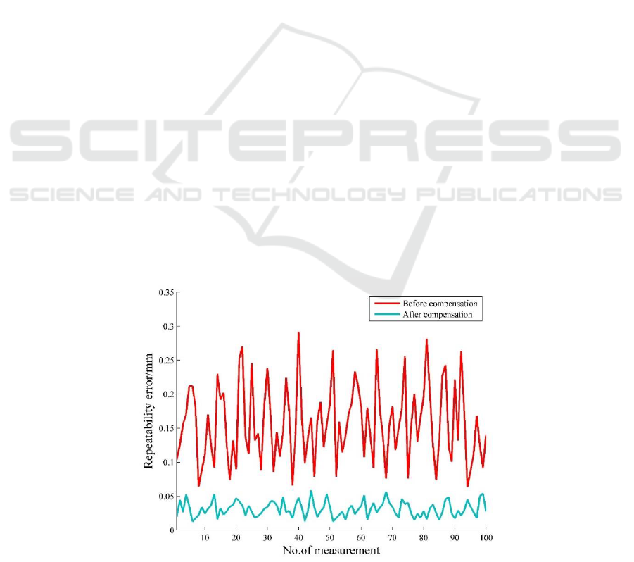
Figure 3. Repeatability error of the single cone-shape hole before and after compensation.

ICVMEE 2019 - 5th International Conference on Vehicle, Mechanical and Electrical Engineering

214

Figure 4. Length measurement errors before and after compensation.

Figure 3 shows the single point repeatability

error before and after model compensation. Let the

average of each set of measurement data be the true

value. It can be seen from the figure that the average

value of the single point repeatability error using the

AACMM is 0.1782 mm, and the average value of it

after the dynamic model compensation is 0.0383

mm. Figure 4 is a length measurement error diagram.

The average length measurement error is reduced

from -0.0681 mm m (before compensation) to -

0.0085 mm (after compensation).

5 CONCLUSION

The source of measurement error of the AACMM is

analyzed, due to the lack of the unified error

calculation formula, a dynamic error compensation

method based on MSA-BP for AACMM is proposed.

The BP neural network is used as the error

compensation model of the AACMM, the weight of

which is optimized by adopting the modified

simulated annealing algorithm, which improves the

convergence speed and operation efficiency. The

simulation results show that the average value of the

repeatability error based on the parameter calibration

is 0.1782mm. After compensation of the MSA-BP

model, the average value of the repeated error is

0.0383mm. The dynamic error compensation model

presented in this paper can effectively improve the

accuracy of the AACMM and has good engineering

application value.

ACKNOWLEDGEMENTS

This paper was supported by Anhui Natural the

Science Foundation (No.1908085ME134), by Anhui

Key Research and Development Plan Project

(No.1804a09020094) and by the key research

project of Natural Science in Anhui University

(No.KJ2018A0054, KJ2018A0060).

REFERENCES

ACERO R., BRAU A., SANTOLARIA J., et al.

Verification of an AACMM using a laser tracker as

reference equipment and an indexed metrology

platform[J]. Measurement, 2015, 69: 52- 63.

Cao Q S, Zhu J, Gao Z F, et al. Design of Integrated Error

Compensating System for the Portable Flexible

CMMs[M]// Computer and Computing Technologies

in Agriculture IV. Springer Berlin Heidelberg,

2010:410-419.

Fedorov V G. Six-axis coordinate measuring machines [J].

Measurement Techniques, 2008, 51(7):724-725

Feng X G, Xu C, Zhang J Y, et al. The establishment and

testing of a model called virtual AACMM [J]. Journal

of Chongqing University, 2016, 39(06):135-140.

Markov B N, Sharamkov A B. The Use of the Results of

Calibration of Faro Arm Coordinate-Measuring

Machines for Use in Comparative Estimation of Their

Precision Capabilities [J]. Measurement Techniques,

2014, 57(8):870-874.

Dynamic Error Compensation Model of Articulated Arm Coordinate Measuring Machine

215

Romdhani F, François Hennebelle, Ge M, et al.

Methodology for the assessment of measuring

uncertainties of AACMMs [J]. Measurement Science

& Technology, 2015, 25(25):125008.

SANTOLARIA J., AGUILAR J.J.,YAGUE J.A., et al.

Kinematic parameter estimation technique for

calibration and repeatability improvement of

AACMM[J]. Precision Engineering, 2008, 32(4): 251-

168.

Santolaria J, José-Antonio Yagüe, Roberto Jiménez, et al.

Calibration-based thermal error model for AACMMs

[J]. Precision Engineering, 2009, 33(4):476-485.

Xing H L, Bo C, Zu R Q. The calibration and error

compensation techniques for an Articulated Arm

CMM with two parallel rotational axes [J].

Measurement, 2013, 46(1):603-609.

ZHANG T, DU L, DAI X. Test of Robot Distance Error

and Compensation of Kinematic Full Parameters [J].

Advances in Mechanical Engineering, 2014, 2014

(22):1-9.

Zhao H N, Yu L D, Jia H K, et al. A New Kinematic

Model of Portable Articulated Coordinate Measuring

Machine [J]. Applied Sciences, 2016, 6(7):181.

Zheng D T, FEI Y T. Research on Spatial Error Model of

Flexible Coordinate Measuring Machine [J]. Journal

of Mechanical Engineering, 2010, 46(10):19-24. (In

Chinese)

Zheng D T, Fei Y T Zhang M. Research on functional

networks of flexible coordinate measuring machine

modelling [J]. Journal of Electronic Measurement and

Instrument, 2009, 23(04): 33-37. (In Chinese)

ICVMEE 2019 - 5th International Conference on Vehicle, Mechanical and Electrical Engineering

216