Topological Approach for Finding Nearest Neighbor Sequence in Time

Series

Paolo Avogadro

and Matteo Alessandro Dominoni

Universit

a Degli Studi di Milano-Bicocca, Viale Sarca 336/14, 20126, Milano, Italy

Keywords:

Time Series, Anomaly, Discord, Nearest Neighbor Distance.

Abstract:

The aim of this work is to obtain a good quality approximation of the nearest neighbor distance (nnd) pro-

ﬁle among sequences of a time series. The knowledge of the nearest neighbor distance of all the sequences

provides useful information regarding, for example, anomalies and clusters of a time series, however the com-

plexity of this task grows quadratically with the number of sequences, thus limiting its possible application.

We propose here an approximate method which allows one to obtain good quality nnd proﬁles faster (1-2

orders of magnitude) than the brute force approach and which exploits the interdependence of three different

topologies of a time series, one induced by the SAX clustering procedure, one induced by the position in time

of each sequence and one by the Euclidean distance. The quality of the approximation has been evaluated

with real life time series, where more than 98% of the nnd values obtained with our approach are exact and

the average relative error for the approximated ones is usually below 10%.

1 INTRODUCTION AND

RELATED WORKS

The large amount of data produced by sensors im-

plies that human analysis of time series needs to be

supported by machine learning techniques. One of

the ﬁrst problems encountered at the time of compar-

ing sequences within a time series is that their length

can span few hundreds of points, and for this rea-

son some form of dimensionality reduction becomes

propaedeutic for further investigations. From this

point of view the symbolic aggregate approximation

(SAX) algorithm (Lin et al., 2003) has proven to be

very effective, as it scales linearly with the size of

the time series, and provides efﬁcient clustering. For

these reasons it has been used as the basis of a large

number of works on the ﬁled (Keogh, 2019). During

the analysis of a time series one often looks for se-

quences which carry particular signiﬁcance. For ex-

ample, anomaly search in time series is a particularly

active research ﬁeld (Chandola et al., 2009), among

the many anomaly concepts, the idea of discords and

a pioneering method for ﬁnding them was introduced

by (Keogh et al., 2005). One of the limitations of dis-

cord search is that the length of the sequences is an

https://orcid.org/0000-0001-5170-4479

https://orcid.org/0000-0001-8481-6311

input parameter, however a priori a researcher does

not know the length of an anomaly. In order to over-

come this problem it has been proposed to use the

Kolmogorov complexity of the symbolic sequences

obtained with the SAX procedure to deﬁne a new con-

cept of anomaly called RRA which produces similar

results compared to discord search (Senin et al., 2014)

(Senin et al., 2018) and it also has the advantage of

being much faster than HOT SAX. At the other side

of the spectrum one might be interested in ﬁnding re-

peated patterns in a time series, for example in the

form of motifs (Chiu et al., 2003) (Patel et al., 2002)

(Lin et al., 2002).

Many of the indicators which allow to character-

ize a time series are obtained by calculating the Eu-

clidean distance between the sequences of a time se-

ries, and in fact the number of calls to the distance

function is often employed for assessing the speed

of an algorithm (Senin et al., 2018). In this respect

a complete knowledge of the distances of all the se-

quences introduces a wealth of information which can

be subsequently used for different primitives. Follow-

ing this perspective the articles of the Matrix Proﬁle

series (Yeh et al., 2016) (Zhu et al., 2016) (and fol-

lowing papers) proposed very fast algorithms which

allow to determine the distance between all the se-

quences of a time series. In this article we thus pro-

vide an approach which allows one to obtain an ap-

Avogadro, P. and Dominoni, M.

Topological Approach for Finding Nearest Neighbor Sequence in Time Series.

DOI: 10.5220/0008493302330244

In Proceedings of the 11th International Joint Conference on Knowledge Discovery, Knowledge Engineering and Knowledge Management (IC3K 2019), pages 233-244

ISBN: 978-989-758-382-7

233

proximate nearest neighbor proﬁle (formally deﬁned

in Sec. 2.1.1) for all the sequences of a time series

which, at variance to the whole matrix proﬁle, is just

the set of all the distances between a sequence and its

closest neighbor. With a good quality nnd proﬁle, it

is possible to make quantitative statistical assessments

regarding the properties of the time series and obtain

new forms of indicators such as the one deﬁned in

(Avogadro et al., ).

2 THREE DIFFERENT

TOPOLOGIES

In this section we detail three topologies of a time se-

ries (intended as notions of neighborhood):

• The Euclidean topology: which determines the

values of nnd

• The SAX topology: which is based on dimen-

sionality reduction and provides a quick grouping

within symbolic sequences

• The time topology: which is naturally determined

by the position of the points of a time series

2.1 Topology Induced by the Euclidean

Metric

The Euclidean distance between two sequences pro-

vides useful insights regarding their similarity. In par-

ticular, if one considers a sequence of s points as a

s−dimensional vector, it becomes straightforward to

use the Euclidean distance to deﬁne clusters of se-

quences, and as a result, to ﬁnd anomalies or recurrent

patterns. We denote with S

the sequence of length s,

where the ﬁrst point of the sequence is at time k. The

point of the sequence S

is denoted as s

. Accord-

ing to this notation, the Euclidean distance between

two sequences (S

and S

) is obtained with:

d(S

, S

) =

∑

n=1



− s



(1)

It is useful to remind that the order of neighbors (e.g.

the nearest neighbor, the second nearest neighbor, ...)

does not change by applying a monotone function

to this quantity (only the nearest neighbor distance

changes). This in turn implies that the same nearest

neighbor is obtained by using the Euclidean distance

or, for example, the d

distance (where no square root

is performed):

, S

) =

∑

n=1



− s



2.1.1 Terminology

• The nearest neighbor distance of a sequence S

deﬁned as:

nnd(S

) = min

j:|i− j|≥s

d(S

, S

), (2)

where the index j runs on all of the possible val-

ues within the search space U, as long as they ex-

clude self matches (|i − j| ≥ s). The concept of

non self match (Keogh et al., 2005) is necessary

to avoid “spurious” low values of nnd because of

partly overlapping sequences.

• The nnd proﬁle is the set of all the possible nnds of

a given search space. An example of nnd proﬁle

is displayed in Fig. 5 (left).

• The nnd density is obtained by dividing in bins

the range of all the possible nnd values and count-

ing the number of sequences which belong to each

bin. As an example, the discord belongs to the

righter-most bin, since, by deﬁnition, it has the

highest nnd value.

It should be noted that the concept of discord is

strictly linked to the search space U (the set of all the

sequences on which the minimization takes place). In

general, since the procedure for obtaining the nnd of

a sequence S is a minimization process, an increase

of the search space can only lead to a decrease of the

nnd. In detail, given two search spaces such that U

⊂

it is true that:

nnd

(S) ≥ nnd

(S). (3)

2.2 SAX Topology

The SAX algorithm (Lin et al., 2003) allows to pro-

duce a quick clusterization of a time series. Two

sequences can, in fact, be considered as neighbors

according to the SAX topology, if they belong to

the same cluster (a.k.a. symbolic sequence or s-

sequence). Notice that this topology is different from

the one induced by the Euclidean distance, since two

sequences can belong to two different SAX clusters

(e.g. they are not close according to SAX), but they

can be closest neighbors according to the Euclidean

metric (and vice versa). In order to understand this, it

might be useful to summarize the SAX procedure:

• Each sequence is fragmented in sub-sequences of

a given length (i.e. a 56 points sequence can be

divided in 7 consecutive sub-sequences, each of 8

points.

KDIR 2019 - 11th International Conference on Knowledge Discovery and Information Retrieval

234

• From each of these sub-sequences, the algebraic

average value is extracted and collected (piece-

wise aggregate approximation or PAA). This tech-

nique allows to pass from a sequence to a re-

duced sequence (r-sequence) of points, where this

r-sequence is smaller than the original one. Each

point of the r-sequence is an average of the points

of the original sequence.

• All the possible values of the averages are further

grouped in intervals (the number of intervals is the

dimension of the alphabet associated to the SAX

procedure) and each interval is assigned to a letter.

For example, let’s consider a sequence composed

of 20 points; we decide to group them in 5 sub-

sequences (each of 4 points). The correspond-

ing r-sequence contains only 5 points which are

then converted into a 3 letters alphabet, where

the letters are obtained with the following vocab-

ulary: [0, 3) → a, [3, 5) → b, [5, 8] → c (consid-

ering that all the points of the r-sequences lay

in the interval [0, 8]). As a result the sequence

34433013225661872103 turns into the symbolic

sequence babca:

sequence 3, 4, 4, 3, 3, 0, 1, 3, 2, 2, 5, 6, 6, 1, 8, 7, 2, 1, 0, 3

r-sequence 14/4, 7/4, 15/4, 22/4, 6/4

r-sequence 3.5, 1.75, 3.75, 5.5, 1.5

s-sequence b a b c a

Thanks to SAX, sequences giving rise to the same

the symbolic sequence are naturally grouped together.

The s-sequences are thus natural clusters for the se-

quences.

2.2.1 Curse of Dimensionality

Since the intervals deﬁning the letters are “sharp”, the

nearest neighbor of a r-sequence close to the borders

of its s-sequence (cluster) might be in a neighboring

cluster. A letter, in fact, does not bring the informa-

tion regarding the fact that the average of points is

close to the center or to the borders (where other let-

ters begin).

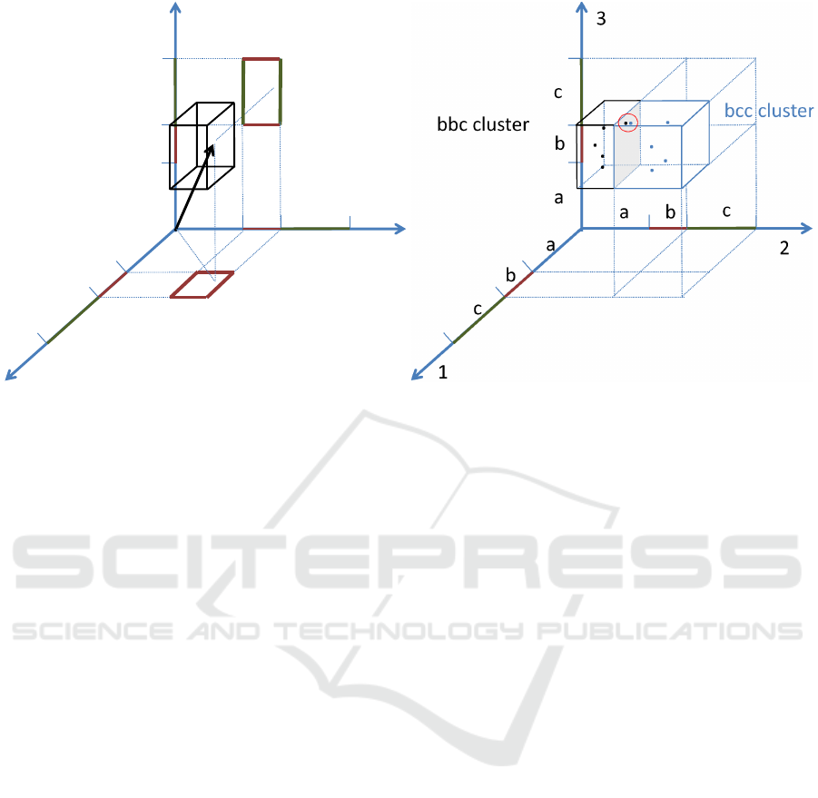
A SAX cluster (symbolic sequence) of n letters

can be approximately seen as a hypercube (Fig. 1),

where each side corresponds to the interval of values

deﬁning a letter. Actually, the object which correctly

represents a SAX cluster is not a hyper-cube since the

intervals don’t need to have the same length. In re-

ality this object is a n-dimensional parallelepiped or

parallelotope (where n is the number of letters of the

sequence). However, since the reasoning related to a

hypercube does not modify the results but it simpliﬁes

the notation, in the following, we will keep on think-

ing in these terms. For high dimensional spaces, most

of the volume of a hypercube is close to its surface,

i.e. the probability to ﬁnd a randomly placed point

close to the borders of the hypercube approaches one

as the number of sides (n) increases to inﬁnity. In or-

der to better understand this fact it is possible to divide

the volume of the hypercube in two concentric parts:

an internal hypercube and an external shell (which is

just the difference between the whole hypercube and

the inner one). It is easy to calculate the inner volume

(where no point has coordinates within a small quan-

tity, ε  l, from one of the faces) since it is an hy-

percube whose side is l − 2ε. The shell between the

inner hypercube and the full one represents the vol-

ume where the points are close to the surface, while

the inner hypercube is the region where the points are

far form the surface. In a scenario of a random dis-

tribution of the points within the symbolic sequence,

the volume of the shell is a good approximation of the

probability of ﬁnding a sequence close to the surface

of the symbolic sequences; vice-versa the volume of

the inner hypercube represent the probability of ﬁnd-

ing a randomly placed point far from the surface. The

ratio of the volume of the inner hypercube and the

full one decreases geometrically with the dimension

of the clusters:

inner volume

volume



l − 2ε



n→∞

−−−→ 0

This implies that, as the dimensionality grows, most

of the volume is located in the external shell of the

hypercube. A point belonging to this region must be

close to at least one of its faces, and thus it is close to a

neighbor hypercube. From this perspective, the SAX

topology becomes less and less likely to approximate

the Euclidean topology as the length of the sequences

increases, since most of the sequences will be close

to the border of the SAX cluster and thus their clos-

est neighbor might be in a neighboring SAX cluster.

Nonetheless it is natural to think that SAX neighbors

are also likely to be Euclidean neighbors (this is in

fact the idea at the basis of HOT SAX (Keogh et al.,

2005)).

2.3 Time Topology

By time topology we simply refer to how distant

in time are the beginnings (or the ends) of two se-

quences, for example the nearest time-neighbors of S

are: S

i−1

and S

i+1

. In general the time distance be-

tween two sequences is simply:

, S

) = |k − j| (4)

Topological Approach for Finding Nearest Neighbor Sequence in Time Series

235

bbc cluster

Figure 1: (Left) A 3-dimensional parallelepiped corresponding to the symbolic sequence bbc, and a point whose coordinates

are averages of the subsequences. (Right) The nearest neighbor of one point of the bbc symbolic sequence is in the next

cluster, bcc, this suggests that the sequences giving rise to those points might be closest Euclidean neighbors but belonging to

different SAX clusters.

3 TOPOLOGY AS A ROAD-MAP

TO FIND THE APPROXIMATE

nnd PROFILE

The idea of this research is to go beyond a brute

force calculation, where one has to scan among all

the Euclidean distances in order to ﬁnd the nearest

neighbor of a sequence. This can be achieved with

a clever selection method which allows to reduce the

total search space and thus the calculation time. This

selection procedure is guided by the different topolo-

gies present in the time series, allowing to aim more

precisely and reducing the problems related with the

curse of dimensionality.

Here we introduce the prescription to ﬁnd the ap-

proximate nnd proﬁle for a quick implementation, in

the rest of the section we will detail the reasons of the

steps. For each sequence S:

1. Perform an extensive nnd search within its own

SAX cluster (Sec. 3.1).

2. Perform an extensive nnd search within its own

SAX cluster, where the size of the alphabet has

been increased from n to n + 1, in respect to step

1 (Sec. 3.2).

3. Execute a search based on time topology (Sec.

3.3). If the nnd up to this point is lower than the

current min(nnd): analyse the next sequence (go

to point 1 with the next sequence).

4. If nnd(S) is still higher than the current min(nnd):

scan the other clusters from the smallest to the

biggest, until the nnd drops below the current min.

When these steps are applied to all the sequences of

the time series, the result is a good approximation of

the nnd proﬁle. Since this strategy runs on an ex-

tended search space compared with the one used by

HOT SAX, it is assured that the discord of the time

series is going to be found. For improving the quality

of the approximate nnd proﬁle, this procedure should

be repeated a few times (10 in the case of the results

of Sec. 4, thus ensuring to ﬁnd the ﬁrst 10 discords).

In order to avoid useless calculations (Bu et al., ), if a

sequence cannot be the discord (because its nnd value

is too low), we skip points 1, 2 when calculating the

discord or above.

The quality of the resulting approximated nearest

neighbor proﬁle will be analysed in Sec. 4. As a refer-

ence, we will now consider the HOT SAX algorithm,

and we will detail how to modify it in order to follow

the procedure just outlined and the reason for these

steps.

HOT SAX.

Let’s consider the approximate nnd proﬁle obtained

with an application of HOT SAX (Keogh et al., 2005).

HOT SAX is a successful algorithm which allows to

ﬁnd anomalies in time series. The idea of this algo-

rithm is to ﬁnd those sequences which are particularly

KDIR 2019 - 11th International Conference on Knowledge Discovery and Information Retrieval

236

different (according to the Euclidean distance) from

all the others: the discords. The discord is deﬁned as

the sequence of the time series which has the maxi-

mum value of nnd. A brute-force discord search re-

quires two nested loops (and thus it is quadratic in

time with the number of sequences). The outer loop

runs on all the sequences. For each sequence S

of the

outer loop, the inner loop runs on all the sequences S

(| j − i| ≥ s), in order to ﬁnd the nnd(S

). The inner

loop is the minimization process needed to ﬁnd the

nearest neighbor. At the opposite, the external loop is

a maximization process aimed at ﬁnding the sequence

for which the nnd is the highest.

The discord sequence is the one with the highest

value of nnd, while the k

discord is deﬁned as the

sequence with the highest nnd in a restricted search

space, which excludes all the sequences which (par-

tially) overlap with any of the previous (k − 1)

dis-

cords. The core idea of the HOT SAX algorithm is to

provide a smart method to exit from the inner loop, in

order to dramatically reduce the execution time. This

is done by re-ordering both the inner and the outer

loops.

At the beginning a SAX clusterization is per-

formed. The outer loop is re-ordered by positioning

at ﬁrst small (SAX) clusters and at the end the biggest

ones. For each sequence of the outer loop, the mini-

mization procedure (for ﬁnding the nearest neighbor

distance of the sequence under observation) begins

by scanning those sequences which are in the same

SAX cluster, and for this reason they are good close

neighbor candidates. If a cluster contains only few se-

quences, it can be seen as an almost empty space and

it is a likely region where to ﬁnd isolated sequences.

This reordering implies that, after a very few steps of

the outer loop the system will have found a good dis-

cord candidate, i.e. a sequence with a high value of

nnd. At this point as soon as the present nnd value of

a sequence (calculated in the inner loop) drops below

the actual highest nnd value, we are sure that that se-

quence cannot be a discord and it is possible to skip

the rest of the minimization process.

The rationale of these choices is that small (SAX)

clusters (in the limit containing only one sequence)

are good places where to ﬁnd anomalies. The nnd

of a sequence of a small cluster will likely be high

(and it is better to search for it at the beginning in

order to have high nnd to confront with); while, on

the contrary, big clusters of sequences will contain

sequences with small nnd. Once the ﬁrst sequences

have been calculated, since they are likely to be good

discord candidates, for the remaining ones, it will be

very likely that the inner loop quickly returns approx-

imate nnd values lower than the actual best discord

candidate. At this point the rest of the inner loop can

be skipped since we are sure that the sequence under

investigation cannot be the discord. These smart or-

derings, in practice, allow to skip most of the inner

loops reducing greatly the complexity of the calcu-

lation. Clearly the execution speed depends on the

time series under consideration, however this algo-

rithm has proven to be extremely efﬁcient in many

practical cases. HOT SAX is thus essentially based

on comparing two different kinds of topologies, the

one induced by the Euclidean metric and the one of

the SAX procedure.

At the end of a HOT SAX calculation each se-

quence has an approximate neighbor (the one at the

time of exiting the inner loop) which determines an

approximate nnd. An approximate proﬁle obtained in

this way as in Fig. 3 (left), however, is very differ-

ent from the exact one of Fig. 5 (left). This is not a

surprise, since the purpose of the algorithm is exactly

to exit from the minimization procedure in order to

avoid useless calculations.

3.1 Extensive nnd Search within the

SAX Cluster of Origin

Let’s introduce here the ﬁrst modiﬁcation of HOT

SAX which improves the nnd proﬁle. Since the code

exits from inner loop as soon as the nnd of a se-

quence is below the current maximum, following the

SAX-Euclidean topology connection, in order to ob-

tain lower values of nnd, it is rather straightforward to

force the calculation to continue for all the sequences

of the same SAX cluster. If the connection between

SAX and Euclidean topology was perfect, this modi-

ﬁcation would assure to ﬁnd the exact nearest neigh-

bor of each sequence. This in practice cannot hap-

pen. The Euclidean distance does induce a notion of

“closeness” however it does not deﬁne automatically

a clusterization.

The rationale of scanning the whole cluster where

the sequence belongs is that, if the sequence under

investigation is close to the center of the SAX cluster,

the Euclidean neighbor has a high chance of being

within the cluster itself. This procedure, is likely to

return the exact nearest neighbor for sequences which

are common within the time series (and thus belong

to big clusters).

3.2 Modifying the Size of the SAX

Alphabet

Because of the curse of dimensionality (Sec. 2.2.1),

for r-sequences near the border of their cluster there is

Topological Approach for Finding Nearest Neighbor Sequence in Time Series

237

a high chance that the closest neighbors might belong

to a different s-sequence (see Fig. 1).

There is a ﬁrst easy cure for this problem. It is pos-

sible, in fact, to apply the SAX procedure two times

in order to produce different symbolic sequences. For

example the second time increasing by 1 the num-

ber of letters of the alphabet for the symbolic repre-

sentation. This prescription, in fact, moves the bor-

ders among the letters, so r-sequences close to the

borders have a high probability of being relocated

in other clusters (maybe containing their true neigh-

bors). Let’s consider a context where the alphabet

contains three letters associated to the following inter-

vals: [0, 3) −→ a; [3, 5) −→ b; [5, 8] −→ c. If the sec-

ond coordinates of two r-sequences are respectively

2.99 and 3.01 the corresponding letters would be a

and b (although these coordinates are very close). For

example:





3.95

2.99

7.21





→









;





3.82

3.01

7.38





→









(5)

By using an alphabet of 4 letters, however, the

intervals associated to each letter would move and

the two points would likely be associated to the

same letter, thus increasing the probability to ﬁnd the

Euclidean nearest neighbor within the same cluster:

[0, 2) −→ a; [2, 4) −→ b; [4, 6) −→ c; [6, 8] −→ d.

The new symbolic sequences associated to the two r-

sequences are:





3.95

2.99

7.21





→









;





3.82

3.01

7.38





→









(6)

Notice that changing the size of the alphabet used

for the symbolic representation does not change the

sequence under investigation, in this way each se-

quence belongs to two (or more if applied many

times) different SAX clusters, where the probability

to ﬁnd the closest Euclidean neighbor increases. This

procedure increases the size of the search space where

we can apply the minimization for ﬁnding the nnd

of each sequence, thus increasing the probability to

ﬁnd a better approximation of the exact value. The

drawback of this procedure is to further slow down

the search (since it increases the search space for each

sequence). Since the two clusters might contain over-

lapping sequences it is useful to keep track of the ones

already checked in the ﬁrst part of the algorithm and

avoid doing the same calculations two times.

3.3 Time for a More Accurate Search

By applying the steps of Sec. 3.1 and Sec. 3.2 it is

possible to obtain a nnd proﬁle which becomes closer

to the exact one, however it is possible to notice that

there is still quite a big number of “suspicious” spikes,

for example in Fig. 4 (left). Up to this point we have

been exploiting the connection between SAX and Eu-

clidean topology. For a further improvement of the

nnd proﬁle, it could be tempting to perform an ex-

tensive search also on the neighboring SAX clusters.

This approach however has two main problems.

• The curse of dimensionality implies that the num-

ber of neighboring clusters grows geometrically,

and there is no simple technique to understand if

any of them is better than the others.

• The amount of sequences to be searched becomes

very big thus rendering the approximate search

not valuable.

As a solution we propose to exploit the time topol-

ogy, which, at this point, can provide useful sugges-

tions regarding the position of close neighbors for

each sequence. Let’s consider the nearest neighbor

distance as a function of the index of the sequence i,

nnd(S

), where i runs over all sequences of the time

series. If the time series shows a certain degree of

regularity, we can expect that also nnd(S

) should be

pseudo-smooth (but for the points where there are true

anomalies). By pseudo-smooth we mean that, it is

possible to obtain upper bounds for nnd(S

i+1

) as a

function of nnd(S

) (and vice-versa). The reason is

rather simple, and in order to show it we will make

use of the d

distance instead of the Euclidean one,

since it allows to get rid of the square root (but the

order of the distances does not change). We will de-

note with p

, where i is the time, the single points of

the time series. With this notation, if the length of

the sequences is s = 10, the last point of sequence

is p

= s

. Let’s consider a sequence, S

, and

its Euclidean nearest neighbor located, for example,

at time i + k (where k is higher than the length of

the sequence s, to prevent a self-match condition), in

this case nnd(S

) = d

, S

i+k

). The nearest neighbor

distance of the next sequence, S

i+1

, is related with

nnd(S

), by Eq 7.

nnd(S

i+1

) ≤ d

i+1

, S

i+k+1

) = nnd(S

) + (p

i+s

− p

i+s+k

)

− (p

− p

i+k

)

(7)

• The ﬁrst inequality of Eq. 7 holds because, by def-

inition, nnd(S

i+1

) is the minimum among all the

distances between S

i+1

and all the other sequences

of the time series.

KDIR 2019 - 11th International Conference on Knowledge Discovery and Information Retrieval

238

• the second part of Eq. 7 is true because of the deﬁ-

nition of the d

distance function, which is a sum-

mation of squares: d

, S

i+k

) =

∑

j=1,s

i+ j

−

i+k+ j

)

If one compares the two distances:

, S

i+k

) = (p

− p

i+k

)

+ (p

i+1

− p

i+k+1

)

+ ...

+(p

i+s−1

− p

i+k+s−1

)

i+1

, S

i+k+1

) = (p

i+1

− p

i+k+1

)

+ ...

+(p

i+s−1

− p

i+k+s−1

)

+(p

i+s

− p

i+k+s

)

• It is easy to notice that the ﬁrst and the last ad-

dend are the only differences between the two dis-

tances, and by hypothesis nnd(S

) = d

, S

i+k

In detail the value of (p

i+s

− p

i+k+s

)

− (p

− p

i+k

)

in Eq. 7 determines whether the inequality implies a

strict limit or not. Since, by deﬁnition, the sequences

beginning at time i and at time i + k are the closest

neighbors, it seems reasonable to expect that the parts

of the time series which follow these two sequences

might resemble each other and thus be close in terms

of Euclidean distance. The information provided by

Eq. 7 is not restricted to the case in which one knows

the exact nnd(S

), but it can be used also in the case

in which the nnd(S

) is approximated, simply provid-

ing a looser upper bound on the value of nnd(S

i+1

Moreover this is true not only from one sequence to

the next one, but a similar relation exists also for the

previous sequence. At this point we have noticed

that time topology can provide good hints on where

to search for nearest neighbors, once an approximate

nnd proﬁle is already present.

This reasoning follows the same basic idea of

the HOT SAX procedure applied to a different

topology, i.e. to provide a hint regarding where to

ﬁnd Euclidean neighbor of a sequence. With a motto,

a sequence could “say”:

The Euclidean-neighbor of my time-neighbor,

is likely to be a time-neighbor of my Euclidean

neighbor.

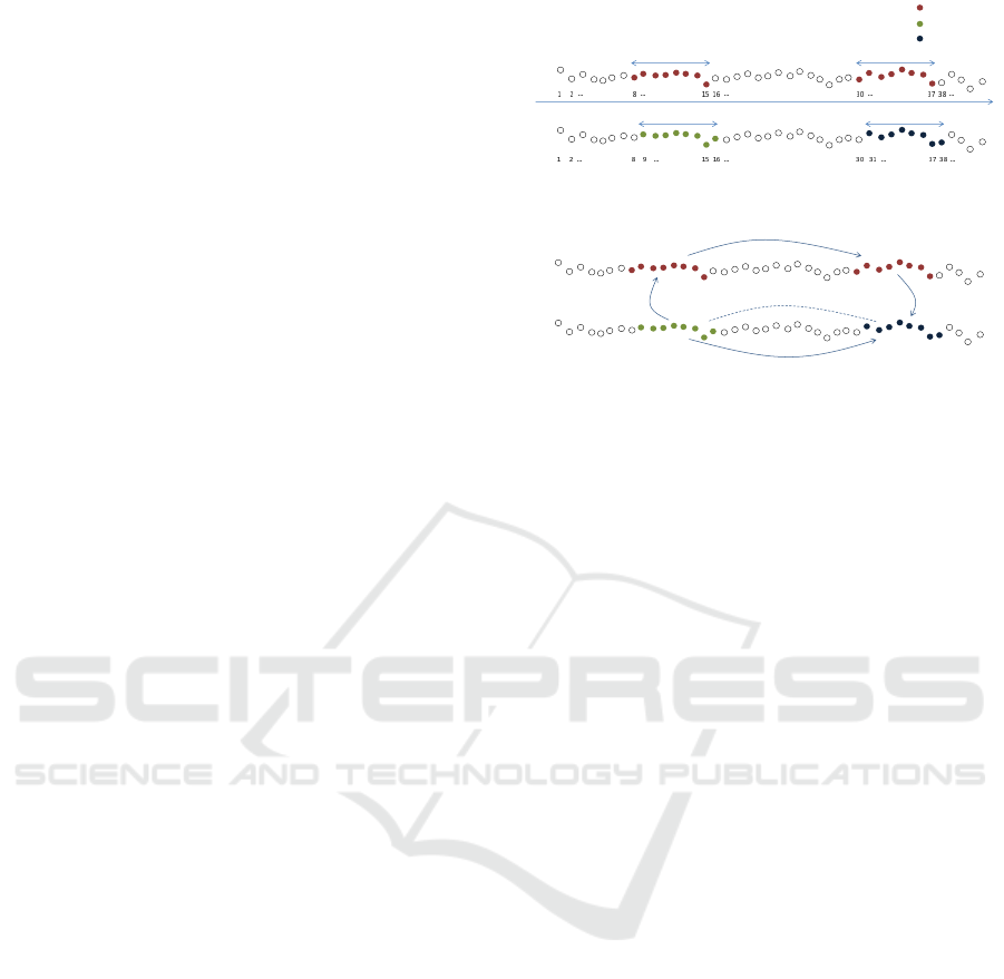
An example of the utilization of the procedure is

shown in Fig. 2, and here synthesized:

• S

is a sequence of length 8. Its Euclidean neigh-

bor has been found within those sequences which

share the same same SAX cluster, in particular is

8+22

• The (approximate) nnd of sequence S

(which is

the time-neighbor of S

) among its SAX neigh-

bors, is much higher than nnd(S

), not following

the constraints of Eq. 7. This is suspicious, since

we expect the nnd proﬁle to be rather smooth (but

for the anomalies).

8+22

9+22

SAX

time

Euclidean

not SAX

cluster A

cluster B

cluster C

Clusters

Exploiting different topologies:

Figure 2: Different kinds of neighborhood: (top ﬁgure) Se-

quence S

and S

are time-neighbors (but they belong to

two different SAX clusters, the red and the green one).

Sequence S

and S

8+22

belong to the same SAX cluster

(the red one), moreover this latter sequence is the clos-

est Euclidean neighbor of the former. Sequence S

(be-

cause of the curse of dimensionality) does not belong to the

same cluster as its closest Euclidean neighbor, S

9+22

, and

there would be no reason to check the distance of the two,

however (bottom ﬁgure) thanks to the following passages:

time

−−→ S

9−1

SAX

−−−→ S

9−1+22

time

−−→ S

9−1+22+1

we can guess

that S

and S

9+22

are likely Euclidean neighbors.

• S

9+22

does not belong to the same SAX cluster

as S

(it belongs to a neighbor cluster, due to the

curse of dimensionality). SAX clustering, in this

case, does not provide good suggestions on where

to search for a good Euclidean neighbor of se-

quence S

• However, thanks of the time topology it is possi-

ble to say that S

9−1+22+1

is a good candidate for

being a close Euclidean neighbor of S

as shown

in Fig. 2 (the summation of the index of the pos-

sible neighbor sequence has not been carried out

in order to emphasize the three passages to obtain

it: time, SAX, and time again).

Clearly it is possible to check on both time direc-

tions in order to improve the quality of the results.

It is also possible to do more loose checks where one

takes into account, not just the ﬁrst time neighbors,

but also more time-distant sequences (up to time dis-

tance= 10 in the present article). This implies that,

for sequence S

, we ﬁrst check the nearest neighbor of

i+ j

( j ≤ 10), denoted with S

. Later, in order to im-

prove nnd(S

), we calculate d(S

, S

l− j

). Actually in

the present implementation we select the sequences to

be checked with a simple heuristic, namely only if the

nnd calculated up to that point presents a non-smooth

behavior (i.e. Eq. 7 is not respected).

Topological Approach for Finding Nearest Neighbor Sequence in Time Series

239

200

400

600

800

1000

1200

1400

0 50000 100000 150000 200000

nnd

sequence time index

200

400

600

800

1000

1200

1400

0 50000 100000 150000 200000

nnd

sequence time index

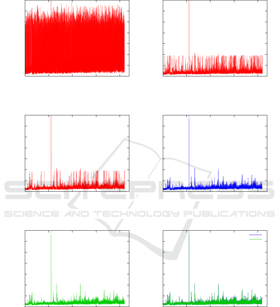
Figure 3: (Left) Approximate nnd proﬁle for all the sequences, obtained with HOT SAX. (Right) The nnd proﬁle obtained by

extending the search space in order to include the whole cluster where each sequence belongs.

200

400

600

800

1000

1200

1400

0 50000 100000 150000 200000

nnd

sequence time index

200

400

600

800

1000

1200

1400

0 50000 100000 150000 200000

nnd

sequence time index

Figure 4: (Left) Approximate nnd proﬁle, obtained with the extended search space including two different kinds of SAX

clusters (with 3 and 4 letters alphabets respectively). (Right) The nnd proﬁle calculated including also the time-topology.

200

400

600

800

1000

1200

1400

0 50000 100000 150000 200000

nnd

sequence time index

200

400

600

800

1000

1200

1400

0 50000 100000 150000 200000

nnd

sequence time index

Approximated nnd

Exact nnd

Figure 5: (Left) Brute force calculation of the exact nnds. (Right) Both the exact (green line) and time-topology approximated

nnd proﬁles (blue line). Since the approximation obtained with the help of time topology is very close to the exact calculations,

the two curves are essentially identical; only a closer look, as in Fig. 7 (right), can allow to distinguish the differences.

4 VALIDATION

In this section we evaluate to which extent the ex-

act nnd proﬁle can be matched with the topologically

approximated one, and what is the gain in terms of

speed. In detail, let’s consider the nnd proﬁle ob-

tained in ﬁve different cases, where each search space

includes the previous one:

KDIR 2019 - 11th International Conference on Knowledge Discovery and Information Retrieval

240

0 40000 80000 120000 160000 200000

Brute-Force/approximate time

Number of sequences

-0.005

0.005

0.01

0.015

0.02

0.025

0.03

0.035

0 50 100 150 200

fraction

nnd

topologically approx. nnd distribution

exact nnd distribution

difference

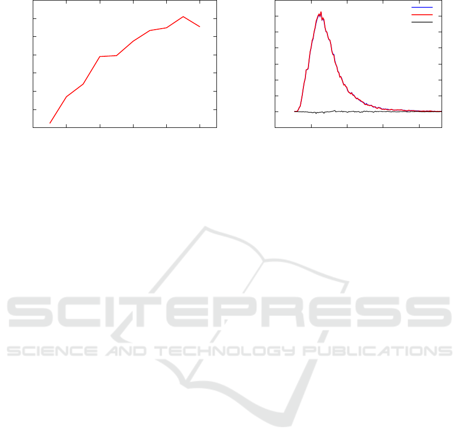
Figure 6: (Left) Ratio of the execution speed of the brute force algorithm and the topological approach for calculating the

nnd proﬁle as a function of the size of the time series to be analysed. In particular we analysed chunks of increasing size

of ECG300. (Right) The topologically approximated nnd densities and the exact one are very similar, and shown here along

with their difference. The interval of nnd values spans from about 0 to about 1400, in order to improve readability, in this

picture, we show values of nnd up to 231.3 since they exhaust 99.5% of the cumulative distribution function, and they allow

to see the main differences between the two densities.

1. The approximate nnd values resulting from the

application of the HOT SAX algorithm is shown

in Fig. 3 (left).

2. Extending the nnd search to all the sequences of

the same cluster produces the approximate nnd of

Fig. 3 (right).

3. Extending the nnd search to all the sequences of

the cluster obtained by using one more letter in the

alphabet returns the nnd proﬁle of Fig. 4 (left).

4. Using also the time topology for the nnd search

provides a clear improvement as of Fig. 4 (right).

5. The results of the exact calculation associated to

the brute force algorithm is in Fig. 5 (left).

In Fig. 5 (right) we show both the exact and the topo-

logically approximated nnd proﬁles for a direct vi-

sual comparison. The time series under consideration,

ECG300, belongs to the MIT-BIH ST change database

available at Physionet (Goldberger et al., e 13). It is

the ECG of a person, sampled 536976 times. In the

pictures, for a better readability of the images we limit

the series to 210000 points (however when taking into

account the accuracy of the approximation we con-

sider all the points). The parameters of the HOT SAX

search are:

• Sequence length: 56 points

• Alphabet size: 3 letters

• 8 points are used to form one letter (which implies

that each sequence/cluster of 56 points contains 7

letters).

It is clear that the approximate nnd proﬁle re-

turned by HOT SAX (Fig. 3 on the left) is useless

for obtaining statistics. This is normal, since the ap-

proach of HOT SAX is to skip all the calculations

which are not necessary for ﬁnding discords, and not

to try to produce good quality nnds. A clear improve-

ment appears if we modify HOT SAX, by forcing it

to run over all the sequences of the cluster associated

to a sequence, as in Fig. 3 (right). In this case, the

algorithm does not exit the loop as soon as the cur-

rent value of the nnd drops below the actual best dis-

cord candidate (as it would do with a normal applica-

tion of HOT SAX), but it keeps on updating the nnd

associated to the sequence. Unfortunately, because

of the curse of dimensionality we can also expect

that many sequences with small Euclidean distance

should be present in neighbor SAX clusters, but the

number of such clusters grows exponentially with the

length of the r-sequences. An easy remedy is to per-

form two times the SAX procedure with two differ-

ent alphabets, i.e in the present example we explored

SAX clusters obtained with 3 letters and with 4 let-

ters. With this approach each sequence belongs to two

different clusters (s-sequences), moreover, since the

range where the letters are chosen passes from even

to odd (or vice versa), it seems reasonable that some

of the neighbors of the r-sequence (which were just

outside of the borders of the ﬁrst SAX cluster) might

fall inside the second SAX cluster. It is worth remem-

bering that the clusters are based on the r-sequences,

and this induces further uncertainty regarding the fact

that two sequences belonging to the same SAX clus-

ter are also Euclidean neighbors. In Fig. 4 (left) there

is the result of this extension which shows a clear im-

provement of the nnds (we remind that the approx-

imate nnds are always greater or equal to the exact

Topological Approach for Finding Nearest Neighbor Sequence in Time Series

241

100

150

200

250

300

350

400

450

66000 66200 66400 66600 66800 67000 67200 67400 67600 67800

Two kinds of clusters

Three topologies

100

150

200

250

300

350

400

450

66000 66200 66400 66600 66800 67000 67200 67400 67600 67800

Three topologies

Exact calculation

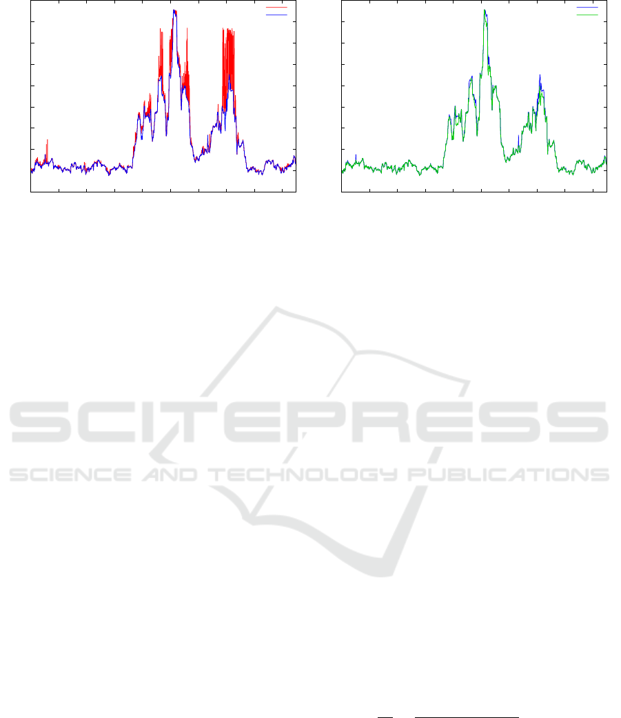
Figure 7: (Left) Detail of the nnds obtained after applying the three topology search (blue) and using two SAX clusters (red).

(Right) Detail of the nnds obtained with the exact calculation (gray) and after applying the three topology search (blue).

Table 1: Comparison of the results of the application of the

topologically approximated nearest neighbor distance pro-

ﬁle to real time series (Goldberger et al., e 13) (Laguna

et al., 1997) and a brute force calculation. The ﬁles sel con-

tain 225000 points, while the bidmc15 series 60000. The

subscripts (

and

) refer to the column of the ﬁles

under investigation, second, third, etc. The speedup is ob-

tained as the ratio of the number of calls to the distance

function of the brute force algorithm and the number of calls

of our approximate algorithm.

ﬁle name % of exact nnds Err speedup

sel0606

99.6 0.05 83

sel0606

99.5 0.05 116

sel102

98.8 0.05 40

sel102

99.7 0.06 26

sel123

98.8 0.05 32

sel123

99.2 0.04 14

bidmc15

99.6 0.15 5

bidmc15

99.8 0.09 30

bidmc15

98.4 0.05 40

bidmc15

98.9 0.06 58

ones, since the only difference among the two is re-

lated to the search space where the minimization takes

place, which is restricted in the case of the approxi-

mate values). At this point one has obtained a good

approximation of the nnd proﬁle, however with a de-

tailed comparison of the approximate nnds and the

exact ones, Fig. 7 (left), it is possible to notice that

the former proﬁle presents many spikes, while the ex-

act proﬁle is more “smooth”. This is an indication

that the curse of dimensionality is still creating prob-

lems and another search mechanism needs to be intro-

duced. The three topology idea ﬁts perfectly this ap-

proach and, by extending the search as per Sec. 3.3,

one obtains the nnd proﬁle of Fig. 4 (right) which

is very close to Fig. 5 (left). At the end, in ﬁgure

5 (right) we compare the exact and the topologically

approximated nnd proﬁle.

In order to better understand the relation between

the the time approximated nnd density and the exact

one, we show them in Fig. 6. Also in this case the dif-

ferences are so small to be almost unnoticeable. We

obtained the nnd densities by dividing the values of

the possible nnds in 1000 bins and for each bin we

counted the number of sequences with a nnd falling

within its limits. The difference among the two den-

sities is also shown for an improved readability. The

topologically approximated nnd density is so close to

the exact one that it can replace it for practical pur-

poses, and in particular when searching for statistical

properties of the nnd proﬁle (Avogadro et al., ).

Fig. 7 (left) shows a detail of the nnd proﬁle calcu-

lated with and without the time topology. It is clearly

visible a high number of spikes which correspond to

poor quality values of the nnd. When passing from

the topologically approximated nnd to the exact one

as in Fig. 7 (right), it is particularly visible that the

differences are more limited both in terms of quantity

and magnitude.

For a quantitative evaluation of the topologically

approximated nnd proﬁle we counted the amount of

exact nnds calculated over the total. In the case of

ECG300 the exact nnd value has been obtained for

98% of the sequences. The average fractional error

of the approximate nnds has been obtained as:

Err =

∑

i=1

nnd

) − nnd(S

)

nnd(S

)

= 3.1 · 10

−2

(8)

Where nnd

) is the approximated nnd value asso-

ciated to the sequence S

, and N

is the amount of se-

quences for which only an approximate nnd has been

found (2% of the total number of sequences). Notice

that there is no reason to use the absolute value, since

nnd

) ≥ nnd(S

) ∀i, the approximated distances are

in fact always greater or equal than the exact ones

KDIR 2019 - 11th International Conference on Knowledge Discovery and Information Retrieval

242

(and in the present case there are no sequences for

which the nnd is exactly 0). In most of the cases (usu-

ally around 99% of the sequences), the numerator of

Eq. 8 is zero. In Table 1 we show the results of the ap-

plication of the topologically approximated nnd pro-

ﬁle for other time series.

5 CONCLUSIONS AND FUTURE

WORKS

When analysing time series, an nnd proﬁle can be

useful in order to characterize the properties of the

sequences, for example to ﬁnd out possible anoma-

lies in the form of discords or recurrent sequences.

Unfortunately a full nnd proﬁle requires calculations

which scale quadratically with the number of points.

In the present article we propose a procedure which

can speed up the process greatly. The idea followed

in this article is to exploit different kinds of neigh-

borhoods for each sequence in order to constrain the

calculations to search spaces where the probability to

ﬁnd the exact neighbor is very high. The three topolo-

gies are: the one introduced by SAX, the time topol-

ogy and the Euclidean topology. The reduced search

space thus obtained allows one to skip most of the cal-

culations while retaining a good accuracy for the nnds

of each sequence.

This is a heuristic selection procedure, and so it is

not possible to provide exact bounds in term of com-

putational complexity. However, the experimental re-

sults we obtained on real data time series are very

interesting since the speed-ups in respect to a brute

force algorithm are between 1 and 2 orders of mag-

nitude. There is also a clear trend indicating that the

ratio between the brute force computational time and

the computational time obtained with the time topol-

ogy increases with the size of the time series under

observation and for this reason our approach becomes

particularly appealing with large time series.

In terms of accuracy, the time-approximated nnd

proﬁles are very close to the exact ones, in the cases

under observation for more than 98% of the sequences

the exact nnd has been found, while for those se-

quences for which just an approximate nnd has been

found, the values are close (≈ 10%) to the correct

ones. It should be emphasized that, due to the nature

of the time-approximated nnd proﬁle (which essen-

tially extends the search space of the HOT SAX algo-

rithm) the results automatically include highest nnds

(corresponding to the discords of the time series).

An interesting result implied by exploiting the

time topology is Eq. 7, which expresses an upper

bound for the nnd of a sequence, once the nnd of a

time neighbor of that sequence is known. In practice

this implies that, once an approximate nnd proﬁle has

been obtained, it is very easy (linear with the size of

the time series) to check if some of the approximate

nnds are particularly distant from their correct value.

In summary, this approach allows to diminish sig-

niﬁcantly the amount of calculations needed to obtain

the nnd proﬁle of a time series at a reasonable loss of

precision. In the present literature the state of the art

is represented by the algorithms of the Matrix Proﬁle

series (Yeh et al., 2016), however they scale quadrat-

ically with the length of the time series and they also

provide information which might be difﬁcult to uti-

lize (they allow to obtain the distance from all the se-

quences while often times only the nearest neighbors

play an important role in determining the properties

of a sequence).

Future works include the application of MASS al-

gorithm which exploits the Fast Fourier Transform

to speed up the calculation of the distances (Mueen

et al., 2017) which is at the basis of (Yeh et al., 2016),

and it is known to greatly speed up the calculation of

distances between sequences.

It is possible to exploit, with minor modiﬁcations,

the procedure provided by this work in order to obtain

approximations of the second, third,..., k-th neighbors

of a sequence and we are in the process of implement-

ing and testing them for an even more complete pro-

ﬁle of the main properties of each sequence.

We are also implementing the time topology to

speed up the calculation of discords.

REFERENCES

Avogadro, P., Palonca, L., and Dominoni, M. A. Online

anomaly search in time series: signiﬁcant online dis-

cords. under review.

Bu, Y., Leung, T.-W., Fu, A. W.-C., Keogh, E., Pei, J., and

Meshkin, S. WAT: Finding Top-K Discords in Time

Series Database, pages 449–454.

Chandola, V., Banerjee, A., and Kumar, V. (2009).

Anomaly detection: A survey. ACM Comput. Surv.,

41(3):15:1–15:58.

Chiu, B., Keogh, E., and Lonardi, S. (2003). Probabilis-

tic discovery of time series motifs. In Proceedings

of the Ninth ACM SIGKDD International Conference

on Knowledge Discovery and Data Mining, KDD ’03,

pages 493–498, New York, NY, USA. ACM.

Goldberger, A. L., Amaral, L. A. N., Glass, L., Hausdorff,

J. M., Ivanov, P. C., Mark, R. G., Mietus, J. E.,

Moody, G. B., Peng, C.-K., and Stanley, H. E.

(2000 (June 13)). PhysioBank, PhysioToolkit, and

PhysioNet: Components of a new research resource

for complex physiologic signals. Circulation,

101(23):e215–e220. Circulation Electronic Pages:

Topological Approach for Finding Nearest Neighbor Sequence in Time Series

243

http://circ.ahajournals.org/content/101/23/e215.full

PMID:1085218; doi: 10.1161/01.CIR.101.23.e215.

Keogh, E. (Accessed 11 July 2019). Welcome to the sax.

https://www.cs.ucr.edu/ eamonn/SAX.htm.

Keogh, E., Lin, J., and Fu, A. (2005). Hot sax: efﬁciently

ﬁnding the most unusual time series subsequence. In

Proceedings of the Fifth IEEE International Confer-

ence on Data Mining (ICDM’05), pages 226–233.

Laguna, P., Mark, R. G., Goldberger, A., and Moody, G. B.

(1997). A database for evaluation of algorithms for

measurement of qt and other waveform intervals in the

ecg. Computers in Cardiology, pages 24:673–676.

Lin, J., Keogh, E., Lonardi, S., and Chiu, B. (2003). A sym-

bolic representation of time series, with implications

for streaming algorithms. In Proceedings of the 8th

ACM SIGMOD Workshop on Research Issues in Data

Mining and Knowledge Discovery, DMKD ’03, pages

2–11, New York, NY, USA. ACM.

Lin, J., Keogh, E., Patel, P., and Lonardi, S. (2002). Find-

ing motifs in time series. In Proceedings of the The

2nd Workshop on Temporal Data Mining, the 8th ACM

Int’l Conference on KDD.

Mueen, A., Zhu, Y., Yeh, M., Kamgar, K., Viswanathan,

K., Gupta, C., and Keogh, E. (2017). The fastest sim-

ilarity search algorithm for time series subsequences

under euclidean distance. http://www.cs.unm.edu/

mueen/FastestSimilaritySearch.html.

Patel, P., Keogh, E., Lin, J., and Lonardi, S. (2002). Mining

motifs in massive time series databases. In 2002 IEEE

International Conference on Data Mining, 2002. Pro-

ceedings., pages 370–377.

Senin, P., Lin, J., Wang, X., Oates, T., Gandhi, S., Boedi-

hardjo, A. P., Chen, C., and Frankenstein, S. (2018).

Grammarviz 3.0: Interactive discovery of variable-

length time series patterns. ACM Trans. Knowl. Dis-

cov. Data, 12(1):10:1–10:28.

Senin, P., Lin, J., Wang, X., Oates, T., Gandhi, S., Boedi-

hardjo, A. P., Chen, C., Frankenstein, S., and Lerner,

M. (2014). Grammarviz 2.0: A tool for grammar-

based pattern discovery in time series. In Calders,

T., Esposito, F., H

ullermeier, E., and Meo, R., ed-

itors, Machine Learning and Knowledge Discovery

in Databases, pages 468–472, Berlin, Heidelberg.

Springer Berlin Heidelberg.

Yeh, C. M., Zhu, Y., Ulanova, L., Begum, N., Ding, Y., Dau,

H. A., Silva, D. F., Mueen, A., and Keogh, E. (2016).

Matrix proﬁle i: All pairs similarity joins for time se-

ries: A unifying view that includes motifs, discords

and shapelets. In 2016 IEEE 16th International Con-

ference on Data Mining (ICDM), pages 1317–1322.

Zhu, Y., Zimmerman, Z., Senobari, N. S., Yeh, C. M., Fun-

ning, G., Mueen, A., Brisk, P., and Keogh, E. (2016).

Matrix proﬁle ii: Exploiting a novel algorithm and

gpus to break the one hundred million barrier for time

series motifs and joins. In 2016 IEEE 16th Inter-

national Conference on Data Mining (ICDM), pages

739–748.

KDIR 2019 - 11th International Conference on Knowledge Discovery and Information Retrieval

244