Modeling Concept Drift in the Context of Discrete Bayesian Networks

Hatim Alsuwat, Emad Alsuwat, Marco Valtorta, John Rose and Csilla Farkas

Department of Computer Science and Engineering, University of South Carolina, Columbia, SC, U.S.A.

Keywords:

Concept Drift, Concept Drift Detection, Nonstationary Environments, Bayesian Networks, Latent Variables.

Abstract:

Concept drift is a signiﬁcant challenge that greatly inﬂuences the accuracy and reliability of machine learning

models. There is, therefore, a need to detect concept drift in order to ensure the validity of learned models.

In this research, we study the issue of concept drift in the context of discrete Bayesian networks. We propose

a probabilistic graphical model framework to explicitly detect the presence of concept drift using latent vari-

ables. We employ latent variables to model real concept drift and uncertainty drift over time. For modeling

real concept drift, we propose to monitor the mean of the distribution of the latent variable over time. For

modeling uncertainty drift, we suggest to monitor the change in beliefs of the latent variable over time, i.e.,

we monitor the maximum value that the probability density function of the distribution takes over time. We

implement our proposed framework and present our empirical results using two of the most commonly used

Bayesian networks in Bayesian experiments, namely the Burglary-Earthquake Network and the Chest Clinic

network.

1 INTRODUCTION

In recent years, machine learning models are increas-

ingly used in many real-world applications. A com-

mon challenge for machine learning systems is to

model environments wherein data evolves over time,

a phenomenon that is commonly known as concept

drift (Gama et al., 2014).

Detecting concept drift is crucial and active re-

search in machine learning systems. Concept drift

inﬂuences the accuracy and reliability of machine

learning models. Current approaches to detect con-

cept drift use latent variables (Borchani et al., 2015;

Caba

nas et al., 2018). Latent variables (a.k.a. unob-

served variables) are variables that are not immedi-

ately observed but instead they are inferred from dif-

ferent variables that are observed and directly mea-

sured. An advantage of concept drift detection tech-

niques that are based on using latent variables is that

they tend to estimate the desired effects on the ma-

chine learning models more reliably than traditional

detection techniques. A large number of observable

variables can be aggregated in a model to represent

an underlying concept, making it easier to understand

the data and detect concept drift over time. However,

current efforts for detecting concept drift using latent

variables either limited to contentious Bayesian net-

works (Borchani et al., 2015) or not directly appli-

cable to discrete Bayesian networks (Caba

nas et al.,

2018). In addition, previous efforts for detecting con-

cept drift using latent variables (Borchani et al., 2015;

Caba

nas et al., 2018) are limited to naive Bayes clas-

siﬁers and therefore cannot be used to model concept

drift that involves concepts span over multiple vari-

ables.

In this paper, we propose a technique for detecting

concept drift in the context of discrete Bayesian net-

works using latent variables. Our technique extends

Borchani et al. (Borchani et al., 2015) approach such

that it is directly applicable to discrete Bayesian net-

works. Borchani et al. represent concept drift using

unobserved variables in continuous domains, namely

in conditional linear Gaussian models. In addition to

modeling posterior probability distribution drift, we

propose a new method for modeling uncertainty drift.

The main contributions of this paper are as fol-

lows. We propose a framework for detecting the

presence of concept drift in the context of discrete

Bayesian networks using latent variables. Unlike pre-

viously proposed approaches (Borchani et al., 2015;

Caba

nas et al., 2018) which are limited to naive Bayes

classiﬁers, our framework is applicable to general

Bayesian network models. We use latent variables

to model two types of drifts over time: (1) Posterior

Distribution Drift, and (2) Uncertainty Drift. We de-

velop a modeling technique using latent variables that

is able to detect posterior distribution drift. We pro-

vide a new method for modeling and detecting con-

214

Alsuwat, H., Alsuwat, E., Valtorta, M., Rose, J. and Farkas, C.

Modeling Concept Drift in the Context of Discrete Bayesian Networks.

DOI: 10.5220/0008384702140224

In Proceedings of the 11th International Joint Conference on Knowledge Discovery, Knowledge Engineering and Knowledge Management (IC3K 2019), pages 214-224

ISBN: 978-989-758-382-7

cept drift via modeling uncertainty over time, i.e., the

amount of belief that changes over time.

We have implemented our approach and presented

our empirical results. Our results indicate that our

modeling framework not only is sensitive to changes

in both real concept drift and uncertainty drift but also

can quickly detect the presence of drifts.

The rest of the paper is organized as follows. In

section 2, we present the problem setting. In sec-

tion 3, we present our framework for detecting con-

cept drift using latent variables in discrete Bayesian

networks. In section 4, we extend our modeling

framework into higher dimensions. In section 5 we

present our empirical results. In section 6, we give an

overview of related work. In section 7, we conclude

and brieﬂy discuss ongoing work.

2 PROBLEM SETTING

We focus on modeling concept drift in the context of

discrete Bayesian networks. In a nonstationary en-

vironment, we assume that at each time point t (for

t = 1, 2, . . . ) data arrives in a batch (a.k.a. a window),

which is a collection of cases. Let Batch [A

, . . . , A

]

be the schema of the incoming batch with attributes

, . . . , A

. We assume without loss of generality that

the incoming batches have equal sizes, i.e., each batch

contains n cases. Let Batch t = {case

, . . . , case

} be

a collection of cases (a.k.a. observations or ﬁndings)

that arrives at time t.

case

, case

, . . . , case

| {z }

Batch 1, t = 1

, case

, . . . , case

| {z }

Batch 2, t = 2

, . . .

Each ﬁnding, denoted as case, is over attributes

, . . . , A

and of the form case = < A

, . . . , A

= v

> (or simply can be written as

case = < v

, . . . , v

>), such that v

is the value

of attribute A

(1 ≤ k ≤ m). When a new batch

Batch t + 1 arrives at time point t + 1, the Bayesian

network model can simply be updated using Bayes’

theorem.

To detect the presence of concept drift between two

time points t = i and t = i + 1, we consider two types

of drifts as follows: (1) Posterior Distribution Drift,

and (2) Uncertainty Drift.

(Posterior Distribution Drift; a.k.a. Real Concept

Drift): Posterior distribution drift occurs when the

conditional probability changes on the target variable

whereas the input variables remain unchanged (Gama

et al., 2014). That is, the value of the posterior prob-

ability at time t = i, P

(y | A), is not equal to the

value of the posterior probability at time t = i + 1,

i+1

(y | A).

In Bayesian statistics, Bayes’ theorem can be writ-

ten in a useful form for Bayesian network update

and inference as follows: The posterior probabil-

ity is proportional to the product of the prior prob-

ability and the likelihood (Posterior probability ∝

Prior probability × Likelihood (Lynch, 2007)). Hav-

ing a prior that is conjugate for the likelihood func-

tion will make it mathematically convenient to cal-

culate the posterior distribution since the posterior

distribution will be from the same family of dis-

tribution as the prior (Raiffa and Schlaifer, 1961).

For instance, multiplying a beta-distributed prior,

Beta(α, β), with a binomial-distributed likelihood

function, Binomial(n, θ), yields a beta-distributed

posterior distribution, Beta(q + α, n − q + β), where

n is the total number of cases, and q is the count of

successes (Alsuwat et al., 2018).

In what follows, we consider detecting the pres-

ence of posterior distribution drift in the context of

discrete Bayesian networks with respect to a random

variable X

X that is beta-distributed, which we denote

as X

X ∼ Beta(α, β). We capture the existence of pos-

terior distribution drift by monitoring the mean of the

beta distribution at every time point t = i, denoted as

, i.e., the expected value of X

X at every time point

t = i, E

(

)

), as follows:

= E

(

)

) =

+ α

α + n

+ β

(1)

where n

and q

are the total number of cases and the

count of successes at time t = i, respectively, and hy-

perparameters α, β are greater than or equal to 1.

(Uncertainty Drift): Measuring the amount of un-

certainty in input data is deﬁned as entropy (Shannon,

2001). Uncertainty drift is a variable that reﬂects the

change in beliefs over time. That is, for a random vari-

able X

X, the maximum value that a probability density

function f

(x;α, β) takes at time t = i is not equal to

the maximum value that a probability density func-

tion f

i+1

(x;α, β) takes at time t = i + 1. This kind of

drift is mainly caused by the change in the total num-

ber of observed cases. It is important to point out that

modeling uncertainty drift in the context of Bayesian

networks is powerful as it is a sensitive diagnostic for

detecting real concept drift.

Herein, we consider detecting the presence of un-

certainty drift in the context of discrete Bayesian net-

works with respect to a random variable X

X is beta-

distributed, X

X ∼ Beta(α, β). We capture the existence

of uncertainty drift by monitoring the maximum value

that the probability density function of the beta distri-

bution takes at every time point t = i, which we denote

Modeling Concept Drift in the Context of Discrete Bayesian Networks

215

Table 1: Notations.

Notation Description

h [

[

, .

, A

]

] The schema of incoming batch with attributes A

, ..., A

h i

i A collection of cases that arrives at time i

The j

observation of Batch i

The mean of the posterior probability at time i

The maximum value that the PDF takes at time i

X A random variable

X ∼ Beta(α, β) A random variable that is beta-distributed

X ∼ Dir(α

, . . . , α

) A random variable that is Dirichlet-distributed

as ψ

, as follows:

= max

X=x

(x;α, β, n

, q

)

= f

(

+ α − 1

α + n

+ β − 2

;α, β, n

, q

)

(2)

where n

and q

are the total number of cases and the

count of successes at time t = i, respectively, x is the

mode of the beta distribution (0 ≤ x ≤ 1), and hyper-

parameters α, β are greater than or equal to 1.

In our setting, we iterate over time steps (t =

1, 2, . . . ). At each time point t = i, we use the incom-

ing batch, Batch i, to update the current Bayesian net-

work model. We then use our approaches to detect the

existence of model drift. we assume that the distribu-

tion of the data does not change inside the batch, i.e.,

we capture the presence of model drift across time

steps (t = 1, 2, . . . ) and not within the set of observa-

tions arrives at a particular time point. If the variations

in the values of µ

and ψ

are important, we conclude

that our Bayesian network model has drifted.

We summarize the notations we use in this paper in

Table 1.

3 MODELING CONCEPT DRIFT

USING LATENT VARIABLES

In this section, we present a modeling technique for

detecting concept drift in discrete Bayesian networks.

We explicitly model concept drift using latent vari-

ables. To avoid unnecessary complication, we assume

that only posterior distribution and uncertainty drift

over time, i.e., for each edge A → B in a Bayesian

network model BN

, we detect the existence of con-

cept drift by monitoring the posterior distribution drift

and uncertainty drift of A → B over time.

Our modeling technique for detecting the presence

of concept drift in discrete Bayesian networks is de-

scribed using plate notation as shown in Figure 1. The

fundamental idea of our modeling approach is to add

a latent node for each edge A → B in a given Bayesian

network model BN

. We call this latent node U

. It

is important to point out that for each collection of

observation j of time t, the unobserved node U

added as the child of the observed nodes A

and B

The latent variable U

captures the posterior drift

and the uncertainty drift for each collection of obser-

vations j of time t. It is essential to point to the fact

that both values of observed variables A

and B

con-

tribute to the drift of the latent variable U

as fol-

lows:

(Posterior Distribution Drift): In our modeling

technique presented in Figure 1, the posterior distri-

bution drift of the latent variable U

that is monitored

at each time point t = i is as follows:

= P

| A

, B

)

+ α

+ n

+ β

where n

and q

are the total number of cases and the

count of successes at time t = i, respectively, and

hyperparameters α

, β

are greater than or equal to 1.

(Uncertainty Drift:) In our modeling technique

shown in Figure 1, to capture the uncertainty drift

of the latent variable U

over time, we monitor the

maximum value that a probability density function

(x;α

, β

) of the latent variable takes at each time

point t = i as follows:

= max

X=x

(x;α

, β

, n

, q

)

= f

(

+ α

− 1

+ n

+ β

− 2

;α

, β

, n

, q

)

where n

and q

are the total number of cases and the

count of successes at time t = i, respectively, x is the

mode of the beta distribution (0 ≤ x ≤ 1), and hyper-

parameters α

, β

are greater than or equal to 1.

It is important to emphasize that our modeling

technique, at each time point t = i, receives j obser-

vations where j = 1 to n. These observations are used

to update the Bayesian network model. The latent

variable U

is then used to capture the presence of

KDIR 2019 - 11th International Conference on Knowledge Discovery and Information Retrieval

216

Figure 1: Modeling concept drift with latent variables in discrete Bayesian networks. A

and B

are observed nodes. U

is a

latent (unobserved) node. θ

, θ

, and θ

are model parameters. α

, β

, α

, β

, α

, and β

are model hyperparameters.

posterior drift (i.e., drift in the value of µ

) and uncer-

tainty drift (i.e., drift in the value of ψ

). If the values

of µ

and ψ

vary signiﬁcantly, we conclude that our

Bayesian network model has drifted.

The a priori expected values of concept and uncer-

tainty drifts can be expressed via the prior distribution

for the latent node U

. We use hyperparameters α

and β

to express the prior knowledge that we may

have about concept and uncertainty drifts at a partic-

ular time point.

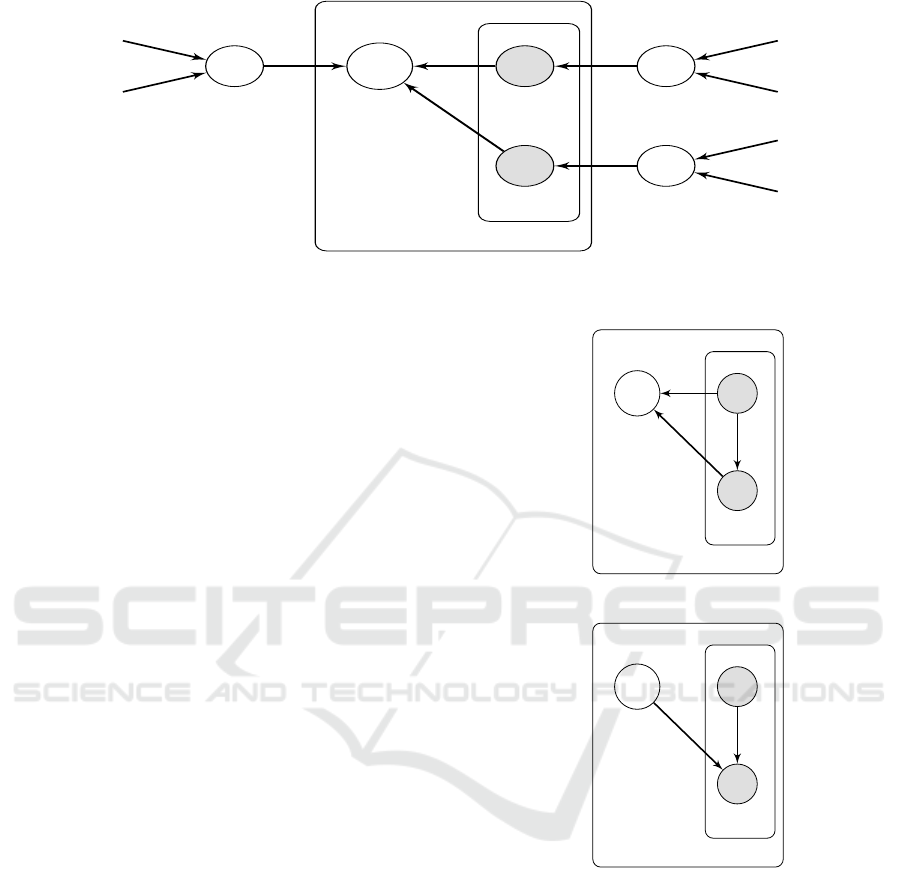
An important point to be made concerning the de-

velopment of our modeling technique for detecting

concept drift (presented in Figure 1) is that it contains

no causal interpretation. We do not place any causal

assumption on the interaction between the observed

variables and the latent variable. Despite the fact that

it is mathematically feasible to build causal and non-

causal modeling techniques (as shown in Figure 2) to

detect the presence of concept drift, it is not neces-

sary to consider causal effects between variables as

these effects are not the main focus of our modeling

approach. For this reason, we tolerate that the inter-

pretation of our modeling approach of concept drift is

merely statistical, i.e., associational.

4 GENERALIZATION OF OUR

FRAMEWORK INTO HIGHER

DIMENSIONS

To expand our modeling framework for variables

with more than two states, we can use the Dirich-

let distribution, which is a continuous multivari-

ate probability distribution. In Bayesian statis-

tics, Dirichlet distribution, which is denoted as

Dir(α

, . . . , α

), is parameterized by r hyperparam-

eters α

, . . . , α

such that α

(1 ≤ i ≤ r) is integer

and α

≥ 1 (Neapolitan et al., 2004). This dis-

tribution is the generalization of the beta distribu-

(a) Non-causal.

(b) Causal.

Figure 2: Options for building a modeling approach for de-

tecting concept drift.

tion for r > 2, i.e., beta is a special case when r =

2. A Dirichlet distributed prior is conjugate for the

likelihood function that is multinomial distributed.

That is, multiplying a Dirichlet-distributed prior,

Dir(α

, . . . , α

), with a multinomial-distributed likeli-

hood function, Multi(w

, . . . , w

, . . . , c

), yields a

Dirichlet-distributed posterior distribution, Dir(α

, . . . , α

+ c

), where α

, . . . , α

are Dirichlet distri-

bution hyperparameters, w

, . . . , w

are Dirichlet dis-

tributed random variables, and c

, . . . , c

are the num-

ber of occurrences of each category.

Modeling Concept Drift in the Context of Discrete Bayesian Networks

217

We focus on detecting the presence of posterior

distribution drift in the context of discrete Bayesian

networks with respect to a random variable X

X =

[

, .

, X

]

] that is Dirichlet-distributed, which we

denote as X

X ∼ Dir(α

, . . . , α

). We capture the exis-

tence of posterior distribution drift by monitoring the

mean of the Dirichlet distribution at every time point

t = i, denoted as µ

, i.e., the expected value of X

every time point t = i, E

(

)

), as follows:

= E

(

)

+ c

all

where α

all

∑

s=1

+ c

and c

is the number of oc-

currences of X

In addition to detecting the posterior drift, we con-

sider detecting the presence of uncertainty drift in the

context of discrete Bayesian networks with respect to

a random variable X

X is Dirichlet-distributed as de-

scribed above. We capture the existence of uncer-

tainty drift by monitoring the maximum value of X

that the probability density function of the Dirichlet

distribution takes at every time point t = i, which we

denote as ψ

, as follows:

= max

(x;α, β, α

all

, c

)

= f

(

+ c

− 1

all

− r

;α, β, α

all

, c

)

where

−1

all

−r

is the mode of the Dirichlet distribu-

tion.

5 EMPIRICAL RESULTS

We have implemented our modeling framework and

tested our approach using two of the most commonly

used example networks in Bayesian experiments,

Burglary-Earthquake Network and Chest Clinic net-

work.

5.1 Burglary-Earthquake Network

The Burglary-Earthquake Network was created by

Pearl (Pearl, 2014) and is a commonly used exam-

ple in Bayesian networks. As shown in Figure 3,

the Burglary-Earthquake Network is a ﬁctitious net-

work that could be used to model an alarm system in

a house. The network consists of ﬁve nodes and four

edges. The nodes are as follows: (1) Node B shows

if there is a burglary, (2) Node E shows whether there

is an earthquake, (3) Node A shows if the alarm goes

off, (4) Node M shows if Mary calls, and (5) Node J

shows if John calls. The causal relations between the

nodes in this network is expressed by directed edges.

For instance, the edge B → A means that burglary may

cause the alarm to be activated and so on. We refer

the readers to (Pearl, 2014) for a full description of

this network.

Figure 3: The original Burglary-Earthquake Network.

We apply our approach for detecting the pres-

ence of concept drift in discrete domains over time

to the Burglary-Earthquake Network. To set up our

experiment, we have implemented this network us-

ing Hugin

Research 8.4. Hugin

case genera-

tor (Madsen et al., 2005; Olesen et al., 1992) is then

used to generate 15 simulated datasets of 1, 000 cases

each. These datasets are named Batch 1 through

Batch 15. During the simulation process of some

datasets, the posterior probabilities are changed in or-

der to simulate the existence of concept drift as fol-

lows: (1) The edge B → A: (i) the posterior prob-

abilities, P(A = F | B = F) and P(A = T | B = F),

are changed during the simulation process of datasets

Batch 3, Batch 7, and Batch 12. (ii) the posterior

probabilities, P(A = T | B = F) and P(A = T | B =

T ), are changed during the simulation process of the

dataset Batch 3. (2) The edge E → A: the poste-

rior probabilities, P(A = F | E = F) and P(A = T |

E = F), are changed during the simulation process

of the dataset Batch 4. (3) The edge A → J: the

posterior probabilities, P(J = F | A = T ), is changed

during the simulation process of the dataset Batch 7.

(4) The edge A → M: the posterior probabilities,

P(M = F | A = F) and P(M = T | A = T ), are changed

during the simulation process of the dataset Batch 7.

In our experiment, we assume that at each time point

t (t = 1, . . . , 15), we receive Batch t which has j in-

stances (we set j = 1, 000 cases).

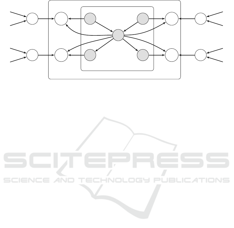
To implement our framework, we added a latent

node for each edge in the Burglary-Earthquake Net-

work. That is, we added latent nodes U

, U

and U

to detect the presence of real concept drift

and uncertainty drift for the edges B → A, E → A,

KDIR 2019 - 11th International Conference on Knowledge Discovery and Information Retrieval

218

a j

Figure 4: Our proposed framework for modeling concept drift with latent variables in the Burglary-Earthquake Network.

A → J, and A → M, respectively, as shown in Fig-

ure 4. We assume that we have no prior knowledge

about concept drift. That is, we assume that all hyper-

parameters of the latent variables, α(.) and β(.), are

equal to 1.

The results of using our framework to detect the

presence of real concept drift and uncertainty drift are

summarized in Table 2 and Table 3, respectively. Note

that values shown in bold in Table 2 and Table 3 indi-

cate the presence of drift. Our framework succeeded

in detecting the existence of real concept drift and un-

certainty drift. We observe that a change in the pos-

terior probability and the uncertainty is reﬂected by a

variation in the evolution of the corresponding latent

variable. For instance, we observe drifts in the pos-

terior probabilities and the uncertainties of the latent

variable U

, namely when U = u | B = F, A = F and

U = u | B = F, A = T , at time points 3, 7, and 12.

We also observe that the posterior and the uncertainty

of the latent variable U

drift at time point 3 namely

when U = u | B = T, A = F and U = u | B = T, A = T .

We observe that our framework is sensitive to

changes in the underlying distribution of data that

newly incoming batches may cause. That is, if the

number of observations in the newly incoming Batch t

at time t is less than the expected number of obser-

vations, then the framework shall report a drop in

the posterior and the uncertainty at time t and vice

versa. For instance, for the edge B → A, namely when

U = u | B = F, A = F, our framework captured a drop

in the posterior and uncertainty drifts in the incom-

ing batch at time point t = 3, Batch 3. This drop is

due to that fact that the number of observed cases in

Batch 3 was less than the expected number of cases.

It should be noted that after each drift, the values

of the posterior and uncertainty will be smoothly re-

increasing/re-decreasing attempting to recover from

the drift. It is also important to point out that if the

number of cases in the newly incoming batch is as ex-

pected, our framework concludes that there is no drift

to anticipate, and thus no action needs to be taken.

Explanations of the other experiments for other edges

trivially follow the explanation of the edge B → A.

All in all, we have shown that our framework

that is based on using latent variables to detect the

presence of concept drift is effective and sensitive to

changes in the underlying distribution of data in non-

stationary environments over time. Our framework

was successfully able to detect the existence of both

real concept drift and uncertainty drift. Our new pro-

posed approach for capturing uncertainty drift is sen-

sitive and useful as it can ensure the occurrence of real

concept drift.

5.2 Chest Clinic Network

The Chest Clinic network, a.k.a. the Visit to Asia

network, was created by Lauritzen and Spielgelhal-

ter (Lauritzen and Spiegelhalter, 1988) and is widely

used in Bayesian network experiments. This network

is a simple, ﬁctitious medical network which could be

employed in a medical facility to diagnose patients as

shown in Figure 5. The Chest Clinic network consists

of eight nodes, which represent random variables, and

eight edges, which indicate the causal relations be-

tween the nodes. A complete description of this med-

ical Bayesian network model is as follows (Lauritzen

and Spiegelhalter, 1988):

Shortness-of-breath (dyspnoea) may be due

to tuberculosis, lung cancer, or bronchitis, or

none of them, or more than one of them. A

recent visit to Asia increases the chances of

tuberculosis, while smoking is known to be a

risk factor for both lung cancer and bronchitis.

The results of a single chest X-ray do not dis-

criminate between lung cancer and tuberculo-

sis, as neither does the presence or absence of

dyspnoea.

Modeling Concept Drift in the Context of Discrete Bayesian Networks

219

Table 2: Results of using our framework to detect the presence of real concept drift in the Burglary-Earthquake Network.

(a) The result of using the latent variable U

to detect the presence of real concept drift for the edge B → A.

Posterior of 1 2 3 4 5 6 7 8 9 10 11 12 13 14 15

B=F,A=F

0.98 0.98 0.94 0.95 0.96 0.96 0.94 0.95 0.96 0.96 0.96 0.94 0.95 0.95 0.96

B=F,A=T

0.006 0.006 0.04 0.032 0.027 0.024 0.04 0.032 0.029 0.027 0.026 0.04 0.032 0.031 0.029

B=T,A=F

0.0005 0.0005 0.003 0.002 0.001 0.001 0.001 0.001 0.001 0.001 0.001 0.001 0.001 0.001 0.001

B=T,A=T

0.01 0.01 0.02 0.01 0.01 0.01 0.01 0.01 0.01 0.01 0.01 0.01 0.01 0.01 0.01

(b) The result of using the latent variable U

to detect the presence of real concept drift for the edge E → A.

Posterior of 1 2 3 4 5 6 7 8 9 10 11 12 13 14 15

E=F,A=F

0.96 0.96 0.96 0.92 0.93 0.93 0.94 0.94 0.94 0.95 0.95 0.95 0.95 0.95 0.95

E=F,A=T

0.01 0.01 0.01 0.06 0.05 0.04 0.04 0.03 0.03 0.03 0.03 0.03 0.02 0.02 0.02

E=T,A=F

0.016 0.015 0.013 0.013 0.013 0.013 0.013 0.013 0.013 0.013 0.013 0.013 0.013 0.013 0.013

E=T,A=T

0.01 0.01 0.01 0.01 0.01 0.01 0.01 0.01 0.01 0.01 0.01 0.01 0.01 0.01 0.01

to detect the presence of real concept drift for the edge A → J.

Posterior of 1 2 3 4 5 6 7 8 9 10 11 12 13 14 15

A=F,J=F

0.93 0.93 0.93 0.93 0.93 0.93 0.93 0.93 0.93 0.93 0.93 0.93 0.93 0.93 0.93

A=F,J=T

0.05 0.05 0.05 0.05 0.05 0.05 0.05 0.05 0.05 0.05 0.05 0.05 0.05 0.05 0.05

A=T,J=F

0.002 0.002 0.002 0.002 0.002 0.002 0.005 0.005 0.005 0.004 0.004 0.004 0.004 0.004 0.003

A=T,J=T

0.01 0.01 0.01 0.01 0.01 0.01 0.01 0.01 0.01 0.01 0.01 0.01 0.01 0.01 0.01

(d) The result of using the latent variable U

to detect the presence of real concept drift for the edge A → M.

Posterior of 1 2 3 4 5 6 7 8 9 10 11 12 13 14 15

A=F,M=F

0.97 0.97 0.97 0.97 0.97 0.97 0.95 0.95 0.96 0.96 0.96 0.96 0.96 0.96 0.96

A=F,M=T

0.01 0.01 0.01 0.01 0.01 0.01 0.01 0.01 0.01 0.01 0.01 0.01 0.01 0.01 0.01

A=T,M=F

0.0059 0.0055 0.0053 0.0052 0.0053 0.0054 0.0055 0.0054 0.0054 0.0054 0.0056 0.0058 0.0059 0.0062 0.0063

A=T,M=T

0.012 0.011 0.011 0.011 0.011 0.010 0.031 0.029 0.027 0.025 0.024 0.023 0.022 0.021 0.020

Table 3: Results of using our framework to detect the presence of uncertainty drift in the Burglary-Earthquake Network.

(a) The result of using the latent variable U

to detect the presence of uncertainty drift for the edge B → A.

Uncertainty of 1 2 3 4 5 6 7 8 9 10 11 12 13 14 15

B=F,A=F

100.12 141.89 92.23 117.43 139.34 160.91 149.16 165.48 181.69 196.20 210.32 200.34 213.09 225.98 238.56

B=F,A=T

176.08 239.53 110.58 143.84 173.97 203.90 179.13 200.81 223.02 243.46 262.87 238.04 255.17 271.71 288.88

B=T,A=F

368.79 736.67 419.45 559.04 659.50 791.25 876.52 1001.63 1075.17 1100.22 1210.16 1272.71 1332.53 1434.97 1489.15

B=T,A=T

120.16 174.42 172.15 209.05 239.86 269.18 270.64 293.38 315.84 335.86 354.83 371.80 389.11 408.88 425.84

(b) The result of using the latent variable U

to detect the presence of uncertainty drift for the edge E → A.

Uncertainty of 1 2 3 4 5 6 7 8 9 10 11 12 13 14 15

E=F,A=F

65.90 93.85 118.30 93.13 110.12 125.49 139.30 152.34 165.06 177.75 189.38 200.50 211.33 222.22 232.59

E=F,A=T

110.77 160.13 203.07 109.76 133.27 156.12 177.12 197.56 217.20 236.51 256.01 274.14 291.73 310.17 327.28

E=T,A=F

103.32 148.89 192.56 224.58 252.62 272.56 291.30 310.42 327.11 348.07 361.79 379.68 396.79 413.21 429.03

E=T,A=T

125.87 174.43 212.23 241.51 270.10 295.95 319.71 339.92 362.59 385.71 407.63 425.18 443.61 461.32 479.88

to detect the presence of uncertainty drift for the edge A → J.

Uncertainty of 1 2 3 4 5 6 7 8 9 10 11 12 13 14 15

A=F,J=F

50.10 70.86 86.79 99.88 111.89 123.16 132.71 142.09 150.68 158.79 166.51 173.99 181.16 188.05 195.24

A=F,J=T

57.31 81.07 98.99 113.62 127.27 139.17 153.76 164.29 174.01 183.21 191.80 200.35 208.54 215.99 223.75

A=T,J=F

271.21 391.32 482.51 559.05 626.30 687.01 459.35 511.28 560.94 608.57 647.27 684.19 726.51 774.78 822.20

A=T,J=T

103.32 146.44 181.48 210.82 236.56 267.54 294.44 313.32 329.78 345.52 364.22 379.68 393.45 408.88 425.84

(d) The result of using the latent variable U

to detect the presence of uncertainty drift for the edge A → M.

Uncertainty of 1 2 3 4 5 6 7 8 9 10 11 12 13 14 15

A=F,M=F

77.67 111.99 136.36 157.73 176.53 194.16 156.79 173.49 187.71 200.94 213.50 225.03 236.74 246.86 257.27

A=F,M=T

120.16 178.65 215.57 247.11 280.35 305.22 330.48 360.53 380.07 394.85 412.89 428.49 445.26 459.79 473.95

A=T,M=F

176.08 250.97 308.18 356.32 391.04 423.24 453.32 487.13 518.79 543.58 562.72 577.34 592.19 603.58 615.41

A=T,M=T

120.16 170.49 209.04 244.26 272.56 305.22 190.01 212.59 232.98 253.50 272.82 291.47 310.56 327.51 345.56

KDIR 2019 - 11th International Conference on Knowledge Discovery and Information Retrieval

220

A S

T L B

X D

Figure 5: The original Chest Clinic network.

We apply our approach for detecting the pres-

ence of concept drift in discrete domains to the Chest

Clinic network. To avoid unnecessary computations,

we use our framework to detect the presence of con-

cept drift of the weakest edge in the Chest Clinic net-

work. Using Alsuwat et al.’s link strength measure,

the edge from A → T is the weakest edge in this net-

work (Alsuwat et al., 2019). Therefore, we employ

our framework to detect the existence of concept and

uncertainty drifts of the edge A → T .

To set up our experiment, we have implemented

this network using Hugin

Research 8.4. Hugin

case generator (Madsen et al., 2005; Olesen et al.,

1992) is then used to generate 15 simulated datasets of

2, 000 cases each. These datasets are named Batch 1

through Batch 15. To simulate the presence of con-

cept drift, we change the posterior probabilities dur-

ing the simulation process as follows: (1) the poste-

rior probability P(T = no | A = no) is changed dur-

ing the simulation process of datasets Batch 4 and

Batch 11. (2) the posterior probability P(T = yes |

A = no) is changed during the simulation process of

dataset Batch 4. (3) the posterior probability P(T =

no | A = yes) is changed during the simulation pro-

cess of dataset Batch 11. (4) the posterior probabil-

ity P(T = yes | A = yes) is changed during the sim-

ulation process of datasets Batch 2 and Batch 10. In

this experiment, we assume that at each time point t

(t = 1, . . . ,15), our framework receives Batch t which

has j observations ( j is set at 2, 000 cases).

To implement our framework, we added a latent

node for the weakest edge in the Chest Clinic net-

work. That is, we added the latent node U

to detect

the presence of real concept drift and uncertainty drift

for the edges A → T as shown in Figure 6. We assume

that we have no prior knowledge about concept drift,

i.e., we assume that the hyperparameters of the latent

variable U

, α

and β

, are equal to 1.

The results of applying our framework to detect

the existence of real concept drift and uncertainty drift

of the weakest edge in the Chest Clinic network are

summarized in Table 4 and Table 5, respectively. Note

that values shown in bold in Tables 4 and 5 indicate

A S

T L B

X D

Figure 6: Our proposed framework for modeling concept

drift of the weakest edge in the Chest Clinic network using

a latent variable.

the presence of drift. Our framework was success-

fully able to detect the presence of real concept drift

and uncertainty drift. We observe that a change in the

posterior probability and the uncertainty is reﬂected

by a variation in the evolution of the latent variable

. For example, we observe drifts in the posterior

probabilities and the uncertainties of the latent vari-

able U

as follows: (1) when U = u | A = no, T = no,

the posterior and the uncertainty drift at time points

4 and 11, (2) when U = u | A = yes, T = no, the

posterior and the uncertainty drift at time point 4,

(3) when U = u | A = no, T = yes, the posterior and

the uncertainty drift at time point 11, and (4) when

U = u | A = yes, T = yes, the posterior and the uncer-

tainty drift at time points 2 and 10.

We observe that our framework is sensitive to

changes in the underlying distribution of incoming

data. Moreover, our framework is able to quickly de-

tect the existence of drifts. Another important obser-

vation is that receiving more observations that belong

to the cell with the highest test statistics value will

reﬂect a higher variation of the evolution of the cor-

responding latent variable and thus will reﬂect a drift

in the posterior and the uncertainty. Overall, we have

shown that our framework that is based on using latent

variables to model concept drift in nonstationary en-

vironments is efﬁcient to detect posterior and uncer-

tainty drifts of the weakest edge in a given Bayesian

network model.

Modeling Concept Drift in the Context of Discrete Bayesian Networks

221

Table 4: Results of using our framework to detect the presence of real concept drift of the weakest edge in the Chest Clinic

network.

Posterior of 1 2 3 4 5 6 7 8 9 10 11 12 13 14 15

A=no,T =no

0.98 0.98 0.98 0.96 0.96 0.97 0.97 0.97 0.97 0.97 0.95 0.96 0.96 0.96 0.96

A=yes,T =no

0.008 0.008 0.008 0.02 0.02 0.01 0.01 0.01 0.01 0.01 0.01 0.01 0.01 0.01 0.01

A=no,T =yes

0.009 0.009 0.009 0.009 0.009 0.009 0.009 0.009 0.009 0.009 0.02 0.02 0.02 0.02 0.02

A=yes,T =yes

0.0009 0.002 0.001 0.001 0.001 0.001 0.0009 0.0009 0.0009 0.001 0.001 0.001 0.001 0.001 0.001

Table 5: Results of using our framework to detect the presence of uncertainty drift of the weakest edge in the Chest Clinic

network.

Uncertainty of 1 2 3 4 5 6 7 8 9 10 11 12 13 14 15

A=no,T =no

137.74 184.65 228.18 197.55 231.22 262.59 290.81 317.06 340.94 361.32 298.71 318.90 338.57 357.81 376.66

A=yes,T =no

205.74 287.02 346.34 236.70 282.12 324.22 363.55 400.53 434.71 468.68 501.12 530.61 558.87 587.62 615.37

A=no,T =yes

183.30 263.10 326.76 374.87 419.77 462.42 499.52 534.05 564.76 595.52 374.68 402.07 429.08 455.05 480.74

A=yes,T =yes

736.31 527.74 751.41 955.80 1144.48 1373.21 1539.98 1696.67 1844.71 1591.53 1716.84 1838.06 1955.52 2069.48 2180.19

6 RELATED WORK

In this section, we will give a brief overview of con-

cept drift, concept drift classiﬁcation, and concept

drift detection methods.

Concept Drift Overview: Applications are increas-

ingly critically dependent on concept schemes for the

semantic interoperability of their data (Wang et al.,

2010). As data evolves over time, real-time data an-

alytics are undermined as the models built to fos-

ter this learning becomes obsolete (

Zliobait

e et al.,

2016). In machine learning, concept drift is a non-

stationary learning problem that develops over time,

often because the training and data application mis-

match in real life scenarios (Moreno-Torres et al.,

2012; Gama et al., 2014). Therefore, concept drift is

associated with a greater probability for prediction in-

accuracies due to misalignment driven by changes in

the statistical properties of the target variable. Most

real-world applications confront some form and de-

gree of shift, which renders this topic highly rele-

vant to the existing and emerging machine learning

community (Moreno-Torres et al., 2012). Concept

drift thus plays a key role in machine learning and

predictive analytics optimization, as adequately ac-

counting for this phenomenon strengthens the over-

all integrity, utility, and functionality of the machine

learning model. Recent surveys on concept drift can

be found in (Iwashita and Papa, 2019; Gama et al.,

2014).

Concept Drift Classiﬁcation: In contemporary sci-

entiﬁc literature, several research has been proposed

to characterize types of concept drift (Webb et al.,

2016; Gama et al., 2014; Iwashita and Papa, 2019).

Webb et al. (Webb et al., 2016) categorized types of

concept drift based on (i) Drift subject, which indi-

cates what aspects of the joint probability drifts over

a period of time, (ii) Drift frequency, which shows

how often concept drift happens during a particular

time, (iii) Drift transition, which indicates the means

wherein the process of changing from one concept to

another occurs, (iv) Drift reoccurrence, which shows

whether or not the occurring concept drift has previ-

ously appeared, and (v) Drift magnitude, which points

out the degree of drift between two time points.

Drift subject is mathematically deﬁned as a

change in the joint probability between two time

points t

and t

as follows: P

(X, y) 6= P

(X, y),

where X is the input variables and y is the target vari-

able (Gama et al., 2014). Drift subject is divided

into two types (Gama et al., 2014): (1) real con-

cept drift, and (2) virtual concept drift. Real concept

drift occurs when the conditional probability changes

on the target variable y whereas the input variables

X remain unchanged, i.e., the posterior probability

changes between two time points t

and t

as fol-

lows: P

(y | X) 6= P

(y | X). Virtual concept drift

occurs when the prior distribution changes between

two time points t

and t

while the posterior prob-

ability remains unchanged (Tsymbal, 2004; Widmer

and Kubat, 1996), i.e., P

(X) 6= P

(X). Real concept

drift is the most important aspect in the category of

drift subject since changes in real concept drift will

degrade the accuracy of the machine learning model

and thus require an update of the model (Kelly et al.,

1999). Therefore, the discussion of this paper is re-

lated to the notion of real concept drift which we refer

to as concept drift.

Concept Drift Detection: One of the challenging

tasks in the context of concept drift is to rapidly de-

tect concept drift and provide a practical measure of

drift magnitude. A variety of concept drift detec-

tion methods have been recently developed. Gama

et al. (Gama et al., 2014) categorized such meth-

ods into four general groups as follows: (1) meth-

ods based on sequential analysis (members of this

group include the Cumulative Sum (CUSUM) and the

Page-Hinkley (PH) (Page, 1954)), (2) methods based

KDIR 2019 - 11th International Conference on Knowledge Discovery and Information Retrieval

222

on statistical process control (members of this group

include the Drift Detection Method (DDM) (Gama

et al., 2004), the Early Drift Detection Method

(EDDM) (Baena-Garcıa et al., 2006), and the Expo-

nentially Weighted Moving Average (EWMA) (Ross

et al., 2012)), (3) methods based on contextual ap-

proaches (a member of this group includes the Splice

system (Harries et al., 1998)), and (4) methods based

on Monitoring distributions on two different time-

windows (members of this group include the Adap-

tive sliding Window (ADWIN) (Bifet and Gavalda,

2007), the Adaptive Cumulative Windows Model

(ACWM) (Sebasti

ao et al., 2017), and SEED Drift

Detector (SEED) (Huang et al., 2014)).

The contribution of this work belongs to the last

one of the four groups. Methods based on monitoring

distributions on two different time-windows are tech-

niques that use statistical tests to compare the distribu-

tions of a ﬁxed reference window on the previous data

and a sliding window on the most recent data (Gama

et al., 2014). Kifer et al. were ﬁrst to propose compar-

ing two detection window distributions in relation to

data streams (Kifer et al., 2004). The team’s presented

algorithms assessed samples taken from two proba-

bility distributions to identify key differences in the

distributions. Another example of such methods was

proposed by (Gama et al., 2006) is the VFDTc sys-

tem, which is an algorithm for mining in nonstation-

ary environments with the ability to detect and adapt

to concept drift. The VFDTc system is used in con-

cept drift resolution through ongoing monitoring of

observed differences between two class-distributions,

including evaluation of: 1) class-distribution when

a node was a leaf, and 2) weighted sum of class-

distributions in the node’s leaf-descendants (Gama

et al., 2006).

Other more recent concept drift detection methods

based on monitoring distributions on two different

time-windows were proposed in (Borchani et al.,

2015) and (Caba

nas et al., 2018). In this work, we

study concept drift detection via comparing distribu-

tions on two different time-windows. We aim to use

latent variables to model and detect concept drift in

the context of discrete Bayesian networks. Borchani

et al. proposed a modeling technique with conditional

linear Gaussian (CLG) that used latent variables to

detect concept drift (Borchani et al., 2015). Their

model is applicable to continuous Bayesian networks

and was applied to continuous domains. Cabanas et

al. proposed a method for detecting concept drift in

discrete streaming data (Caba

nas et al., 2018). Their

proposed preprocessing algorithm transferred discrete

data into continuous data before applying Borchani at

el. model to detect concept drift. However, Cabanas

et al.’s technique is susceptible to data loss and results

in increased processing overhead when used in incre-

mental learning domains.

7 CONCLUSION AND FUTURE

WORK

Detecting changes in the underlying distribution of in-

coming data, a.k.a. concept drift detection, is a vital

and active research area in machine learning systems.

In this paper, we studied the presence of concept drift

in the context of discrete Bayesian networks in non-

stationary environments. We have proposed a frame-

work for modeling concept drift using latent variables

in discrete Bayesian networks. Our modeling tech-

nique using latent variables is capable of detecting

real concept drift and uncertainty drift over time. We

have applied our framework for detecting the pres-

ence of concept drift in discrete domains over time

to the Burglary-Earthquake Network and the Chest

Clinic Network, which are the most widely used net-

works in Bayesian experiments. Our results indicate

that our framework is not only sensitive to changes in

the underlying distribution of incoming data but also

can easily detect the real concept drift and uncertainty

drift over time. Our ongoing work extends these re-

sults to ﬁnd explanations for the changes of the mod-

els. Such explanations will improve our understating

of the evolution of the concept drift. This indeed may

permit to distinguish malicious attacks from natural

model shift. In addition, we aim to acquire an authen-

tic dataset for further experiments and compare our

approach with other approaches that model concept

drift using latent variables.

REFERENCES

Alsuwat, E., Alsuwat, H., Valtorta, M., and Farkas, C.

(2019). Adversarial data poisoning attacks against the

pc learning algorithm. International Journal of Gen-

eral Systems, pages 1–29.

Alsuwat, E., Valtorta, M., and Farkas, C. (2018). How to

generate the network you want with the pc learning

algorithm. In Proceedings of the 11th Workshop on

Uncertainty Processing (WUPES’18), pages 1 – 12.

Baena-Garcıa, M., del Campo-

Avila, J., Fidalgo, R., Bifet,

A., Gavalda, R., and Morales-Bueno, R. (2006). Early

drift detection method. In Fourth international work-

shop on knowledge discovery from data streams, vol-

ume 6, pages 77–86.

Bifet, A. and Gavalda, R. (2007). Learning from time-

changing data with adaptive windowing. In Proceed-

Modeling Concept Drift in the Context of Discrete Bayesian Networks

223

ings of the 2007 SIAM international conference on

data mining, pages 443–448. SIAM.

Borchani, H., Mart

ınez, A. M., Masegosa, A. R., Langseth,

H., Nielsen, T. D., Salmer

on, A., Fern

andez, A., Mad-

sen, A. L., and S

aez, R. (2015). Modeling concept

drift: A probabilistic graphical model based approach.

In International Symposium on Intelligent Data Anal-

ysis, pages 72–83. Springer.

Caba

nas, R., Cano, A., G

omez-Olmedo, M., Masegosa,

A. R., and Moral, S. (2018). Virtual subconcept drift

detection in discrete data using probabilistic graphi-

cal models. In International Conference on Informa-

tion Processing and Management of Uncertainty in

Knowledge-Based Systems, pages 616–628. Springer.

Gama, J., Fernandes, R., and Rocha, R. (2006). Decision

trees for mining data streams. Intelligent Data Analy-

sis, 10(1):23–45.

Gama, J., Medas, P., Castillo, G., and Rodrigues, P. (2004).

Learning with drift detection. In Brazilian symposium

on artiﬁcial intelligence, pages 286–295. Springer.

Gama, J.,

Zliobait

e, I., Bifet, A., Pechenizkiy, M., and

Bouchachia, A. (2014). A survey on concept

drift adaptation. ACM computing surveys (CSUR),

46(4):44.

Harries, M. B., Sammut, C., and Horn, K. (1998). Extract-

ing hidden context. Machine learning, 32(2):101–

126.

Huang, D. T. J., Koh, Y. S., Dobbie, G., and Pears, R.

(2014). Detecting volatility shift in data streams. In

2014 IEEE International Conference on Data Mining,

pages 863–868. IEEE.

Iwashita, A. S. and Papa, J. P. (2019). An overview on con-

cept drift learning. IEEE Access, 7:1532–1547.

Kelly, M. G., Hand, D. J., and Adams, N. M. (1999). The

impact of changing populations on classiﬁer perfor-

mance. In Proceedings of the ﬁfth ACM SIGKDD in-

ternational conference on Knowledge discovery and

data mining, pages 367–371. Citeseer.

Kifer, D., Ben-David, S., and Gehrke, J. (2004). Detecting

change in data streams. In Proceedings of the Thirti-

eth international conference on Very large data bases-

Volume 30, pages 180–191. VLDB Endowment.

Lauritzen, S. L. and Spiegelhalter, D. J. (1988). Local

computations with probabilities on graphical struc-

tures and their application to expert systems. Journal

of the Royal Statistical Society. Series B (Methodolog-

ical), pages 157–224.

Lynch, S. M. (2007). Introduction to applied Bayesian

statistics and estimation for social scientists. Springer

Science & Business Media.

Madsen, A. L., Jensen, F., Kjaerulff, U. B., and Lang, M.

(2005). The hugin tool for probabilistic graphical

models. International Journal on Artiﬁcial Intelli-

gence Tools, 14(03):507–543.

Moreno-Torres, J. G., Raeder, T., Alaiz-Rodr

ıGuez, R.,

Chawla, N. V., and Herrera, F. (2012). A unifying

view on dataset shift in classiﬁcation. Pattern Recog-

nition, 45(1):521–530.

Neapolitan, R. E. et al. (2004). Learning bayesian networks,

volume 38. Pearson Prentice Hall Upper Saddle River,

NJ.

Olesen, K. G., Lauritzen, S. L., and Jensen, F. V. (1992).

ahugin: A system creating adaptive causal probabilis-

tic networks. In Uncertainty in Artiﬁcial Intelligence,

1992, pages 223–229. Elsevier.

Page, E. S. (1954). Continuous inspection schemes.

Biometrika, 41(1/2):100–115.

Pearl, J. (2014). Probabilistic reasoning in intelligent sys-

tems: networks of plausible inference. Elsevier.

Raiffa, H. and Schlaifer, R. (1961). Applied statistical de-

cision theory. Div. of Research, Graduate School of

Business Administration, Harvard Univ.

Ross, G. J., Adams, N. M., Tasoulis, D. K., and Hand,

D. J. (2012). Exponentially weighted moving average

charts for detecting concept drift. Pattern recognition

letters, 33(2):191–198.

Sebasti

ao, R., Gama, J., and Mendonc¸a, T. (2017). Fad-

ing histograms in detecting distribution and concept

changes. International Journal of Data Science and

Analytics, 3(3):183–212.

Shannon, C. E. (2001). A mathematical theory of commu-

nication. ACM SIGMOBILE mobile computing and

communications review, 5(1):3–55.

Tsymbal, A. (2004). The problem of concept drift: deﬁ-

nitions and related work. Computer Science Depart-

ment, Trinity College Dublin, 106(2):58.

Wang, S., Schlobach, S., and Klein, M. (2010). What is

concept drift and how to measure it? In International

Conference on Knowledge Engineering and Knowl-

edge Management, pages 241–256. Springer.

Webb, G. I., Hyde, R., Cao, H., Nguyen, H. L., and Petit-

jean, F. (2016). Characterizing concept drift. Data

Mining and Knowledge Discovery, 30(4):964–994.

Widmer, G. and Kubat, M. (1996). Learning in the pres-

ence of concept drift and hidden contexts. Machine

learning, 23(1):69–101.

Zliobait

e, I., Pechenizkiy, M., and Gama, J. (2016). An

overview of concept drift applications. In Big data

analysis: new algorithms for a new society, pages 91–

114. Springer.

KDIR 2019 - 11th International Conference on Knowledge Discovery and Information Retrieval

224