Text Mining in Hotel Reviews: Impact of Words Restriction in Text

Classification

Diogo Campos

, Rodrigo Rocha Silva

2,3 a

and Jorge Bernardino

1,2 b

Polytechnic of Coimbra - ISEC, Rua Pedro Nunes, Quinta da Nora, 3030-199 Coimbra, Portugal

Centre of Informatics and Systems of University of Coimbra, Pinhal de Marrocos, 3030-290, Coimbra, Portugal

FATEC Mogi das Cruzes, São Paulo Technological College, 08773-600 Mogi das Cruzes, Brazil

Keywords: Text Mining, Sentiment Analysis, Text Cube, Machine Learning, Stemming.

Abstract: Text Mining is the process of extracting interesting and non-trivial patterns or knowledge from unstructured

text documents. Hotel Reviews are used by hotels to verify client satisfaction regarding their own services or

facilities. However, we can’t deal with this type of big and unstructured data manually, so we should use

OLAP techniques and Text Cube for modelling and manage text data. But then, we have a problem, we must

separate the reviews in two classes, positive and negative, and for that, we use Sentiment Analysis technique.

Nevertheless, do we really need all the words of a review to make the right classification? In this paper, we

will study the impact of word restriction on text classification. To do that, we create some words domains

(words that belong to a Hotel Domain). First, we use an algorithm that will pre-process the text (where we

use our created domains like stop words). In the experimental evaluation, we use four classifiers to classify

the text, Naïve-Bayes, Decision-Tree, Random-Forest, and Support Vector Machine.

1 INTRODUCTION

Text Mining is the process of extracting interesting

and non-trivial patterns or knowledge from

unstructured text documents that can be visualized as

consisting of two phases: text refining that transforms

free-form text documents into a chosen intermediate

form, and knowledge distillation that deduces

patterns or knowledge from the intermediate form

(Noel, 2018). Hierarchical Topic Model, Author-

Topic Analysis, Spatio-Temporal Analysis,

Sentiment Analysis, and Multistream Bursty Pattern

Finding are some of the techniques that we can use

for text mining, but in this paper, we will focus on

Sentiment Analysis. Sentiment Analysis is the

process that analysis a statement/opinion of a person

and will determine the sentiment/emotion of that

statement, that could be positive or negative.

Sentiment Analysis is also referred to as emotional

polarity computation (Li and Wu, 2010).

Nowadays, as we work with bigger datasets,

because more people have access to the Internet and

can express their opinions easily, we need to interpret

https://orcid.org/0000-0002-5741-6897

https://orcid.org/0000-0001-9660-2011

and well-understand the data, so we can use a text

cube to organize the data in multiple dimensions and

hierarchies (Liu et al., 2013). In this type of dataset,

we can organize the data in two dimensions, positive

reviews and negative reviews, which is a simple

multi-dimensional, as if we use a Topic Model

technique to organize the data will be a most complex

multi-dimensional cube.

But, in Sentiment Analysis we need to understand

which are the words that influence the accuracy of

this text mining technique, so we create seven-word

restriction models that we will use in text

classification and then compare the results.

To classify the right sentiments in each document

we will use Machine Learning that works very well

when working with text categorization and text

mining techniques as Sentiment Analysis (Sebastiani,

2002). We use four of the most famous Machine

Learning algorithms: Naïve Bayes, Decision Tree,

Random Forest and Support Vector Machine. These

algorithms will classify the text from dataset

“Sentiment analysis wit hotel reviews | 515K Hotel

Reviews Data in Europe | Kaggle, 2017” and try to

442

Campos, D., Silva, R. and Bernardino, J.

Text Mining in Hotel Reviews: Impact of Words Restriction in Text Classiﬁcation.

DOI: 10.5220/0008346904420449

In Proceedings of the 11th International Joint Conference on Knowledge Discovery, Knowledge Engineering and Knowledge Management (IC3K 2019), pages 442-449

ISBN: 978-989-758-382-7

focus each sentence on his own polarity, which can

be positive or negative, a two-class problem.

The main objectives of this work are the

following:

 Compare the results (Accuracy, Memory Used,

Classification Time) of each algorithm and

evaluate which is the better one for this type of

two-way class problem;

 Visualize how each model affect the results and

understands the big outliers between the models

and how can word restriction affect text

classification.

The main innovation of this paper is the

introduction of Word Models that will restrict the text

and provide a better perspective of the impact of those

models in the results. For example, the difference

between have a good classification or not can be

unlocked by a word that is included in a Word Model,

so we thought that could be an important statement to

study and we will focus on Common Words and

Adjectives and try to understand which one provide

us better classifications results.

The remainder of this paper is organized as

follows. In Section 2, we give an overview of related

work on this topic. In Section 3, we present our

experimental methodology (Dataset, Models that we

created, Classification Methods, Text Pre-Process).

Section 4 presents the results of the experimental

evaluation. Section 5 concludes this paper and show

future research issues.

2 RELATED WORK

Many authors used Sentiment Analysis to classify

documents using machine learning approaches, but in

our searches, we couldn’t find one that have tried to

understand how playing with words can affect the text

classification. That is what we propose to do in this

paper, but also discover which is the best machine

learning algorithm to work with this type of dataset

(two-way class).

Gautam and Yadav (2014) compares Naïve

Bayes, SVM and Maximum Entropy on Twitter data.

The authors conclude that Naïve Bayes had better

results than the other two algorithms.

Fang and Zhan (2015) focus on the problem of

sentiment polarity categorization. Despite of using all

four algorithms that we use in our paper; the authors

don’t give enlightening results that we can use to

compare and study the machine learning algorithms.

The work of Sharma and Dey (2012) explores the

applicability of five commonly used feature selection

methods in data mining research (DF, IG, GR, CHI

and Reflied-F) and seven machine learning based

classification techniques (Naïve Bayes, Support

Machine, Maximum Entropy, Decision Tree, K-

Nearest Neighbour, Winnow, Adaboost). The authors

conclude that SVM gives the best performance for

sentiment-based classification and for sentimental

feature selection.

3 EXPERIMENTAL

METHODOLOGY

Fig. 1 shows the overall architecture of the

experimental methodology that is used to the

classification task of this paper. The proposed

methodology is divided into five parts. The first one

consists of choosing the dimension of the dataset that

we going to work and clean it, described in section

3.1. After that, we must do a pre-process of the text,

described in section 3.2. In section 3.3 we will

describe the classification process and in section 3.4

we explain our evaluation process and the comparison

of the results.

Figure 1: Experimental methodology.

Text Mining in Hotel Reviews: Impact of Words Restriction in Text Classiﬁcation

443

3.1 Description of the Dataset

The dataset that we choose for this investigation

(Sentiment analysis wit hotel reviews | 515K Hotel

Reviews Data in Europe | Kaggle, 2017) contains

515,000 customer reviews and a scoring of 1493

luxury hotels across Europe. Meanwhile, the

geographical location of hotels is also provided for

further analysis.

This dataset presents seventeen attributes (“Hotel

Address”, “Additional Number of Scoring”, “Review

Date”, “Average Score”, “Hotel Name”, “Reviewer

Nationality”, “Negative_Review”, “Review Total

Negative Word Counts”, “Total Number of reviews

Positive Review”, “Review Total Positive Word

Counts”, “Total Number of Reviews Reviewer Has

Given”, “Reviewer Score”, “Tags”, “Days Since

Review”, “LAT”, “LNG”), but we only will use 2 of

them, “Positive Review” and “Negative Review”

because this work only requires the use of reviews for

training data, so other attributes aren’t necessary for

this investigation.

For classification task, we select Positive_Review

and Negative_Review and give them a score, positive

and negative, respectively. The review of the user

goes into a string called review, and if a user didn’t

do a review but s/he’s on the dataset we delete

him/her from the training dataset.

There is an example of one review in this dataset.

“This hotel is awesome I took it sincerely because a

bit cheaper but the structure seem in an hold church

close to one awesome park Arrive in the city are like

10 minutes by tram and is super easy The hotel inside

is awesome and really cool and the room is incredible

nice with two floor and up one super big comfortable

room I’ll come back for sure there The staff very

gentle one Spanish man really good.”

3.2 Pre-process of the Text

Online text usually has a lot of noise and

uninformative parts like HTML tags, scripts,

advertisements, and punctuations. So, we need to

apply a process that cleans the text, for example, that

removes that kind of noise to have better

classification results (Haddi, Liu and Shi, 2013).

The first step of this process is to convert all the

instances of the dataset to lowercase, which will allow

to better compare the words with all the models that

are created. Then, we remove HTML tags and

punctuations. After that we can opt by removing stop

words or use our created domains, being that, we need

to remove empty reviews in the end and stemming the

text of the reviews. Now we will specifically explain

the stemming, removing stop words process and in

the end talk about the utilization of our created

domains:

Stemming: this process reduces words to their own

stems. For example, two words, "fishing", "Fisher"

after going into this process are changed to the main

word "fish". In this experimental study, we are using

Porter Stemmer because it is one of the most popular

English rule-based stemmers. Various studies have

shown that stemming helps to improve the quality of

the language model (Allan and Kumaran, 2003;

Brychcín and Konopík, 2015). This improvement

leads to another improvement in the classification

task where the model is being used.

Removing Stop Words: stop word removal is a

standard technique in text categorization (Yang et al.,

2007). This technique manipulates a list of commonly

used words like articles and prepositions, this type of

words doesn't matter to our classification task, so we

are removing them from the text. For this

experimental study, we use a list of common words

of English Language that includes about 100-200

words.

Created Domains: these domains are what make the

difference in our study. We decide to create two

words domains: the first one “Hotel_Domain”, with

596 common hotel words and the second one

“Adjectives”, with 197 adjective words that we can

use about hotels. We use these word domains like the

list of Stop Words, removing or only restrict those

words to the text, so we can compare how the word

restriction works in Sentiment Analysis and Text

Classification.

Eliminate Empty Reviews: as we use our domains to

restrict the text in this pre-processing task, there are

reviews that will be empty so we have to remove them

from the training data that we will consider for train

and test.

Text Transformation (TF-IDF): TF-IDF calculates

values for each word in a document through an

inverse proportion of the frequency of the word in a

document to the percentage of documents the word

appears in (Medina and Ramon, 2015). Therefore,

this algorithm gives more weight and relevance to

terms that appear less in the document comparatively

with terms that appear more frequently. This process

of text transformation must be used because machine

learning algorithms can't work with text features.

3.3 Experiment Models

We use 7 experiment models of words restriction that

we will describe below:

KDIR 2019 - 11th International Conference on Knowledge Discovery and Information Retrieval

444

Model 1: In this model, we remove all the Stop

Words in the document, so for the text classification

we only consider all the words except the Stop

Words.

Model 2: In this model, we only consider the words

that the “Hotel_Domain” contains the text

classification, all other words are removing.

Model 3: In this model, we use the domain of

“Adjectives” to do the words restriction. Basically,

we only consider the words that the “Adjectives”

contains the text classification.

Model 4: This model is a junction of models 2 and 3.

We only consider words that exist on the two domains

that we create.

Model 5: In this model, we use “Hotel_Domains” as

the process of removing Stop Words, but instead of

removing the words of the list of Stop Words, we

remove the words of our common words domain.

Model 6: In this model, we don’t consider any list of

restriction words. We use all words to classify the

text.

Model 7: The last model we use, is a model that

contains the list of Stop Words plus the domain of

common words that we have created. Basically, in

this model, we only consider the words that exist on

these two domains of words.

3.4 Classification Methods

After the pre-process of the text, we need to split the

data in training and test. In this study, we use 80% of

the data for training and 20% for the test which allows

us to better results compare with 70% train and 30%

of test. Then, we use that training data to train the

classifiers that we will explain and used in this

experimental study, and we use the test data to

evaluate them. In the following we will describe the

four algorithms that we used:

Naïve Bayes: this classifier is a well-know and

practical probabilistic classifier that assumes that all

features of the examples are independent of each

other given the context of the class, and independence

assumption. Myaeng, Han and Rim (2006), for

example, a fruit may be considered to be an apple if

it is red, round, and about 3” in diameter. In that

situation, this classifier considers each one of these

“features” to contribute independently to the

probability that the fruit is and apple, regardless of

any correlation between features (Naive Bayes for

Dummies; A Simple Explanation - AYLIEN, 2017).

In the context of text classification this algorithm uses

the Bayes Theorem to calculate the probability of a

document belong to a class as the theorem follows:

𝑃

(

𝐵

𝐴

)

𝑃

(

𝐵

𝐴

)

𝑃

(

𝐴

)

× 𝑃

(

𝐵

)

In these experiments, we use the Multinomial type of

Naïve Bayes classifier with default parameters.

Decision Tree: this classifier uses trees to predict the

class of an instance. A tree is either a leaf node labeled

with a class or a structure consisting of a test node

linked to two or more subtrees. An instance is

classified by starting at the root node of the tree. If

that node is a test, the outcome for the instance is

determined and the process continues using

appropriate subtree. When a leaf is eventually

encountered, it’s label gives the predicted class of the

instance (Quinlan and Quinlan J. R., 1996). We

utilize (random_state=42) for this study.

Random Forest: it is a combination of tree predictors

such that each tree depends on the values of a random

vector sampled independently and with the same

distribution for all trees in the forest. Is a classifier

consisting of a collection of tree-structured classifiers

{h(x,Θ

), k =1, …} where the { Θ

} are independent

identically distributed random vectors and each casts

a unit vote for the most popular class at input x

(Breiman, 2001). In this experimental study, we are

using the criteria of the random forest “gini” and the

number of trees “100”, which provide the best results,

after a couple of tests.

Support Vector Machine (SVM): this classifier is

based on the Structural Risk Minimization principal

from computational learning theory. The idea of

structural risk minimization is to find a hypothesis h

for which we can guarantee the lowest true error

(Joachims, 1998). Basically, SVM is responsible for

finding the decision boundary to separate different

classes, on our case, positive and negative, and

maximize the margins between the hyperplane (line

who separate the classes). On this experimental study,

we will use two models of the SVM Algorithm: RBF

and Linear.

4 EXPERIMENTAL RESULTS

4.1 Algorithms Comparison

First, we will do a comparison between the machine

learning algorithms without using any model, so we

can compare the real performance of the algorithms

and do better conclusions. For this experience we

only use 12500 reviews, because of the time it spends

to do all the experiments and we run each algorithm

five teams and collect the average accuracy,

precision, recall, classification time and memory used

Text Mining in Hotel Reviews: Impact of Words Restriction in Text Classiﬁcation

445

of each one, these metrics that we will explain

following:

Accuracy: is the proportion of correctly classified

examples to the total number of examples, while error

rate uses incorrectly classified instead of correctly

(Mouthami, Devi and Bhaskaran, 2013).

Classification Time: is the time that the text

classification occurs. To get this parameter we use a

function that give us the difference of time between

the start of the classification and the end.

Memory Used: is the memory that is used by all the

experimental methodology process. PID of the

process will give us the memory used in each

classification.

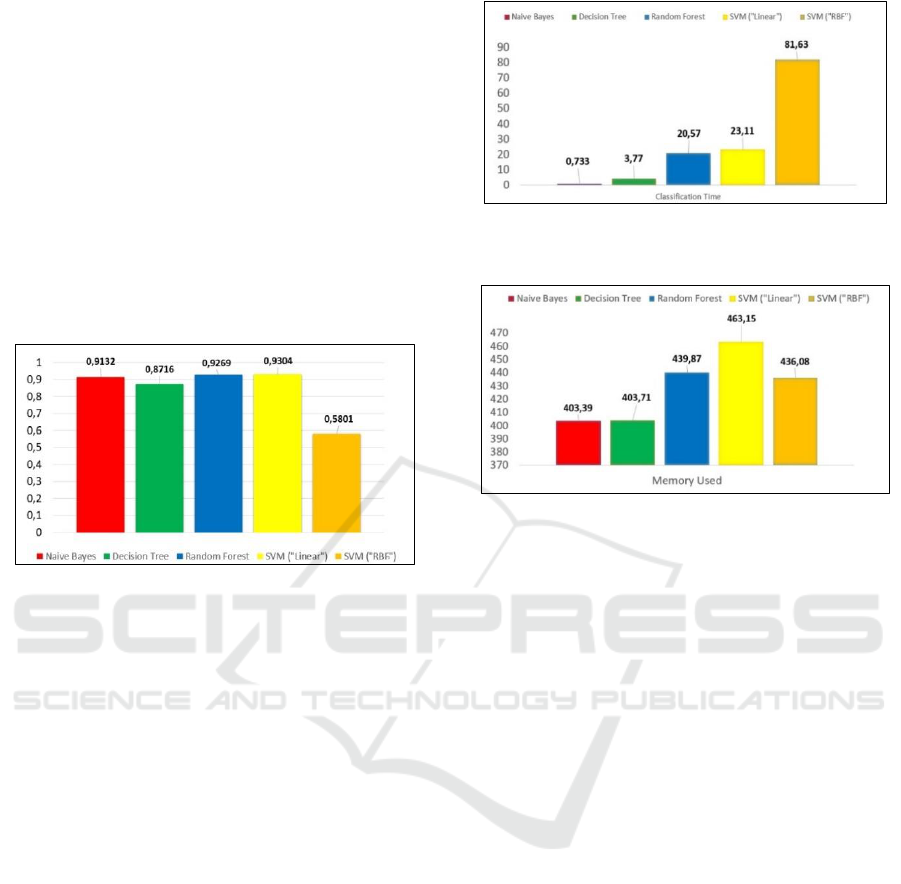
Figure 2: Accuracy comparison between Algorithms.

According to Fig. 2, we can conclude that Support

Vector Machine (“Linear”) has the best performance

in terms of Accuracy with a value of 93,04% versus

92,69% of Random Forest and 91,32% of Naïve

Bayes. Decision Tree with 87,16% and SVM

(“RBF”) with 58,01% came after. Since this dataset

presents a two-way class problem, SVM (“RBF”) has

obvious the worst result because is an algorithm that

works better in problems that don’t be linearly

separable. Naïve Bayes, Decision Tree, Random

Forest have worst results than SVM (“Linear”)

because are simple Algorithms. SVM (“Linear”) is a

most complex algorithm that uses Support Vectors to

optimize the margins between the two classes and that

improve the results in comparison with the simple

algorithms.

According to Fig. 3, Naïve Bayes is the algorithm

that spend less time on text classification, because of

only uses the Bayes Theorem to find the class of the

sentence is a very simple algorithm. In comparison

with the rival algorithms that had better results in

terms of Accuracy, Random Forest and SVM

(“Linear”), Naïve Bayes gives us a way better

classification time than the other two algorithms with

an average of 0.733 seconds because of that

simplicity and that is an advantage if we need or want

to increase the number of training instances.

Figure 3: Classification Time comparison between

algorithms.

Figure 4: Memory Used comparison between algorithms.

According to Fig. 4, we can conclude that Naïve

Bayes is the algorithm that spent less memory in all

classification process with 403,39 Mbytes, with

Random Forest spend more 36,45 Mbytes and SVM

(“Linear”) spend more 59,76 Mbytes.

Based on all these results, we can conclude that,

despite of SVM (“Linear”) has better performance on

Accuracy level, Naïve Bayes is faster and spent less

computer memory to the text classification.

4.2 Models Comparison

In this section, we will show the impact of the words

restriction models that we created had on each

machine learning classifier in terms of accuracy,

classification time and memory used.

4.2.1 Naïve Bayes

Based on Table 1 the model that brings the best

Accuracy value is Model 7, however, values are very

similar to models 1, 3, 5 and 6. We can explain these

results in a fact that these 4 models, do a better job

restricting the text to the right words that can help the

algorithm to find the right call of the review. The fact

that model 7 had the best accuracy value didn’t mean

that is better than the other 3 models that we talk

before. In terms of classification time and memory

used the model 3 has the best values, and that is

because that model only considers the words of the

KDIR 2019 - 11th International Conference on Knowledge Discovery and Information Retrieval

446

domain of adjectives that we created, so the training

data that we will consider will be so much less than

the other models, the algorithm will spend less

memory and the algorithm find faster the right class.

Table 1: Naïve Bayes results: Accuracy, Classification

Time, and Memory used.

Models

Accuracy

Classification

Time (s)

Memory

(MB)

Model 1

0,9134

0,529s

332,88

Model 2

0,6737

0,137s

248,75

Model 3

0,8906

0,105s

237,11

Model 4

0,8125

0,188s

237,80

Model 5

0,9137

0,655s

361,69

Model 6

0,9132

0,733s

398,59

Model 7

0,9165

0,613s

313,40

4.2.2 Decision Tree

As we came to Decision Tree classifier the results that

we get in terms of accuracy that we show in Table 2,

are worse than Table 1, as the model that had better

accuracy was model 3, but the models 1, 5 ,6 and 7

also had good values of accuracy like in Naïve Bayes.

This classifier is more complex that Naïve Bayes, so

the times of text classification increase, despite model

3 had the best result again. The values of memory

used in this classifier are relatively the same as the

Naïve Bayes with model 3 had the best result, with

some ups and downs. The decline of accuracy values

in this algorithm can be explain to the fact this

algorithm only uses one tree to reach the class in the

training review, and sometimes some reviews don’t

have enough words to help the algorithm to find the

class, considering the test review, what doesn’t

happen on Naïve Bayes.

Table 2: Decision Tree results: Accuracy, Classification

Time, and Memory used.

Models

Accuracy

Classification

Time (s)

Memory

(MB)

Model 1

0,8615

3.3s

331,28

Model 2

0,6699

0,304s

243,64

Model 3

0,8761

0,134s

236,09

Model 4

0,7874

0,479s

238,95

Model 5

0,8690

2,98s

370,21

Model 6

0,8716

3,77s

401,76

Model 7

0,8643

3,21ss

312,69

4.2.3 Random Forest

The Random Forest classifier that is an upgrade of the

decision tree classifier as this classifier use multiple

trees to find the right class of the reviews versus the

only one tree classifier Decision Tree, so we can

expect better results in terms of accuracy, but bad

results in terms of classification time, because of the

increase of ramifications and trees, that makes this

algorithm more complex computationally. As we can

see in Table 3, the same models that we refer before

have the best values of accuracy, but in this classifier

model 6 provide us a 92,69% of accuracy, which is

very good, however, we can’t conclude anything from

here of what is the best model of restriction words. In

terms of classification time and memory used model

3 has the best values again and as we said before the

values increase in all models because of the superior

complexity of the algorithm compared with Naïve

Bayes and Decision Tree.

Table 3: Random Forest results: Accuracy, Classification

Time, and Memory used.

Models

Accuracy

Classification

Time (s)

Memory

(MB)

Model 1

0,9054

21,3s

391,13

Model 2

0,6807

4,07s

251,15

Model 3

0,8886

1,13s

248,91

Model 4

0,8074

5,85s

263,90

Model 5

0,9212

17,49s

411,18

Model 6

0,9269

20,57s

438,85

Model 7

0,9087

18,94s

369,77

4.2.4 SVM (“Linear”)

In this section, we will analyse the results of the most

complex algorithm, the support vector machine. We

use the SVM (Kernel =” Linear”) classifier that

provides us the best accuracy results compare to the

other classifiers. However, as the SVM is the most

complex algorithm, it’s normal that the memory that

is used in the process have a slight increasement,

however not in comparison with Random Forest

which is a complex algorithm too, but the time

doesn’t have to, because as this dataset provides us a

two-way class problem, the linear classifier is the

perfect classifier for this type of training data, but as

we use only 12500 reviews for classification we can’t

say that these values are good classification time

results.

Based on Table 4, once again model 6 has the best

accuracy value with 93,04% and model 3 has the best

values of classification time and memory used, as the

memory values are very similar to Decision Tree and

Naïve Bayes and we get the best memory value with

213,59 Mbytes.

Text Mining in Hotel Reviews: Impact of Words Restriction in Text Classiﬁcation

447

Table 4: SVM (“Linear”) results: Accuracy, Classification

Time, and Memory used.

Models

Accuracy

Classification

Time (s)

Memory

(MB)

Model 1

0,9189

19,1s

337,51

Model 2

0,6657

5,75s

225,75

Model 3

0,8771

1,02s

213,59

Model 4

0,8087

5,3s

235,81

Model 5

0,9302

19,76s

361,27

Model 6

0,9304

23,11s

461,88

Model 7

0,9226

13,48s

316,96

4.2.5 SVM (“RBF”)

In this section, we present the results of SVM (Kernel

= “RBF”) classifier. This is not the best classifier to

work with in this type of dataset and two-way class

problems and that explains the bad results that we

have in terms of accuracy and classification time. In

terms of memory used the values are very similar to

Random Forest.

Based on Table 5, model 3 provides us the best

accuracy value with 86,92% and that result can be

explained to the fact that model only consider

adjectives, which are words that can easily help the

algorithm to find the right class. In terms of

classification time and Memory Used the times

increase significatively in this classifier, being that

the memory used results are similar to SVM

(“Linear”), so we can conclude that Kernel RBF is a

bad classifier to use in this type of text of

classification problems, but definitely can be use in

datasets that have more than 2 classes, not linear

problems

Table 5: SVM (“RBF”) results: Accuracy, Classification

Time, and Memory used.

Models

Accuracy

Classification

Time (s)

Memory

(MB)

Model 1

0,5703

61,28s

339,14

Model 2

0,6188

8,38s

225,33

Model 3

0,8692

1,71s

215,79

Model 4

0,7576

10,54s

236,53

Model 5

0,5616

76,02s

365,56

Model 6

0,5801

81,63s

382,24

Model 7

0,5839

45,85s

321,14

5 CONCLUSIONS AND FUTURE

WORK

In this paper, we have proposed several restriction

words models that can help to understand the impact

that words have in text classification. For the

classification task, we use the four of the most

popular machine learning algorithms to work with

Sentiment Analysis and analyse posterior results

based on three measures: Accuracy, Classification

Time and Memory Used.

Our first results have shown that the best

algorithm to work with is Naïve Bayes because Naïve

Bayes spend less time and use less memory to find the

right class than others, despite the Random Forest and

SVM (“Linear”) gives us better accuracy values. That

benefit of spend less time and use less memory will

allow us to growth the training data, continuing with

good accuracy values. However, as Naïve Bayes is

the less complex algorithm, because only uses a

theorem to calculate the probability of a word belong

to a class, it’s difficult to try to improve this accuracy

results, so maybe a good solution is trying to find a

way to improve Random Forest or SVM ("Linear”)

with the otherwise to spend more time and memory

to training data and get results.

In terms of the best restriction words model, after

we compare all of them in the 5 classifiers we made a

conclusion that the model 1, 3, 5, 6, and 7 are the

models that give us the best accuracy results, but

looking more at the models profoundly we think that

models 3 and 5 are the best models that can have a

good impact on text classification with other hotel’s

datasets and they also have good classification time

results and memory values because model 3, which

use only adjectives give us always good classification

results if there is an adjective in the review, this model

reduce the dimension of the review a lot and can work

with the most complex algorithms in terms of

memory and time, model 5 because in that model as

we remove Common Words and the accuracy results

are good we can conclude that common words don’t

affect text classification as much as adjectives and

this is applicable to other datasets.

As future work, we plan to increase the number of

reviews to have a better perspective of the evolution

of results. For example, as we increase the number of

reviews see the growth or the decline of the values.

We also want to join the text mining method topic

model and study what are the most significative

topics that we can take off a review to help the hotels

in a possible search of good or bad reviews of a topic,

or which is the topic with more good/bad reviews.

REFERENCES

Allan, J. and Kumaran, G. (2003) ‘Stemming in the

language modeling framework’, p. 455. doi:

10.1145/860500.860548.

KDIR 2019 - 11th International Conference on Knowledge Discovery and Information Retrieval

448

Breiman, L. (2001) ‘RANDOM FORESTS Leo’, pp. 1–33.

Brychcín, T. and Konopík, M. (2015) ‘HPS: High precision

stemmer’, Information Processing and Management,

51(1), pp. 68–91. doi: 10.1016/j.ipm.2014.08.006.

Fang, X. and Zhan, J. (2015) ‘Sentiment analysis using

product review data’, Journal of Big Data. Journal of

Big Data, 2(1). doi: 10.1186/s40537-015-0015-2.

Gautam, G. and Yadav, D. (2014) ‘Sentiment analysis of

twitter data using machine learning approaches and

semantic analysis’, 2014 7th International Conference

on Contemporary Computing, IC3 2014. IEEE, pp.

437–442. doi: 10.1109/IC3.2014.6897213.

Haddi, E., Liu, X. and Shi, Y. (2013) ‘The role of text pre-

processing in sentiment analysis’, Procedia Computer

Science. Elsevier B.V., 17, pp. 26–32. doi:

10.1016/j.procs.2013.05.005.

Joachims, T. (1998) ‘Text categorization with support ector

machines: Learning with many relevant features’,

Lecture Notes in Computer Science (including

subseries Lecture Notes in Artificial Intelligence and

Lecture Notes in Bioinformatics), 1398, pp. 137–142.

doi: 10.1007/s13928716.

Sharma, A and Dey, S (2012) ‘A Comparative Study of

Feature Selection and Machine Learning Techniques

for Sentiment Analysis’, Proceedings of the 2012 ACM

Research in Applied Computation Symposium, pp. 1–

7. doi: 10.1145/2401603.2401605

Liu, X. et al. (2013) ‘SocialCube: A text cube framework

for analyzing social media data’, Proceedings of the

2012 ASE International Conference on Social

Informatics, SocialInformatics 2012. IEEE,

(SocialInformatics), pp. 252–259. doi:

10.1109/SocialInformatics.2012.87.

Medina, C. P. and Ramon, M. R. R. (2015) ‘Using TF-IDF

to Determine Word Relevance in Document Queries

Juan’, New Educational Review, 42(4), pp. 40–51. doi:

10.15804/tner.2015.42.4.03.

Mouthami, K., Devi, K. N. and Bhaskaran, V. M. (2013)

‘Sentiment analysis and classification based on textual

reviews’, 2013 International Conference on

Information Communication and Embedded Systems,

ICICES 2013. IEEE, pp. 271–276. doi:

10.1109/ICICES.2013.6508366.

Myaeng, S. H., Han, K. S. and Rim, H. C. (2006) ‘Some

effective techniques for naive bayes text classification’,

IEEE Transactions on Knowledge and Data

Engineering. IEEE, 18(11), pp. 1457–1466. doi:

10.1109/TKDE.2006.180.

Naive Bayes for Dummies; A Simple Explanation -

AYLIEN (no date). Available at: http://blog.aylien.com

/naive-bayes-for-dummies-a-simple-explanation/ (Ac

cessed: 30 April 2019).

Noel, S. (2018) ‘Text Mining for Modeling Cyberattacks’,

Handbook of Statistics, 38, pp. 463–515. doi:

10.1016/bs.host.2018.06.001.

Quinlan, J. and Quinlan J. R. (1996) ‘Learning decision tree

classifiers’, ACM Computing Surveys (CSUR), 28(1),

pp. 2–3. Available at: http://dl.acm.org/citation.cfm?id

=234346.

Sebastiani, F. (2002) ‘P1-Sebastiani’, ACM Computing

Surveys, 34(1), pp. 1–47. doi: 10.1145/505282.505283.

Yang, J. et al. (2007) ‘Evaluating bag-of-visual-words

representations in scene classification’, Proceedings of

the international workshop on Workshop on

multimedia information retrieval - MIR ’07, p. 197.

doi: 10.1145/1290082.1290111.

Text Mining in Hotel Reviews: Impact of Words Restriction in Text Classiﬁcation

449