Uncertainty and Fuzzy Modeling in Human-robot Navigation

Rainer Palm and Achim J. Lilienthal

AASS, Dept. of Technology,

Orebro University, SE-70182

Orebro, Sweden

Keywords:

Human-robot Interaction, Navigation, Fuzzy Modeling, Gaussian Noise.

Abstract:

The interaction between humans and mobile robots in shared areas requires a high level of safety especially

at the crossings of the trajectories of humans and robots. We discuss the intersection calculation and its

fuzzy version in the context of human-robot navigation with respect to noise information. Based on known

parameters of the Gaussian input distributions at the orientations of human and robot the parameters of the

output distributions at the intersection are to be found by analytical and fuzzy calculation. Furthermore the

inverse task is discussed where the parameters of the output distributions are given and the parameters of the

input distributions are searched. For larger standard deviations of the orientation signals we suggest mixed

Gaussian models as approximation of nonlinear distributions.

1 INTRODUCTION

Activities of human operators and mobile robots in

shared areas require a high degree of system stabil-

ity and security. Planning of mobile robot tasks,

navigation and obstacle avoidance were major re-

search activities for many years (Khatib, 1985; Firl,

2014; Palm and Lilienthal, 2018). Using the same

workspace at the same time requires adapting the be-

havior of human agents and robots to facilitate suc-

cessful collaboration or support separate work for

both. (O.H.Hamid and N.L.Smith, 2017) present a

general discussion on robot-human interactions with

the emphasis on cooperation. In this context, recog-

nizing human intentions to achieve a particular goal

is an important issue reported by (Tahboub, 2006;

Fraichard et al., 2014; Palm et al., 2016; Palm and

Iliev, 2007). The problem of crossing trajectories be-

tween humans and robots is addressed by Bruce et

al. who describe a planned human - robot rendezvous

at an intersection zone (Bruce et al., 2015). In this

connection the goal to achieve more natural human-

robot interactions is obtained by human-like sensor

systems as they share their functional principle with

natural systems (Robertsson et al., 2007; Palm and

Iliev, 2006; Kassner et al., 2014). Based on an es-

timate of the positions and orientations of robot and

human, the intersections of the intended linear trajec-

tories of robot and human are calculated. Due to sys-

tem uncertainties and observation noise, the intersec-

tion estimates are also corrupted by noise. In (W.Luo

et al., 2014) and (J.Chen et al., 2018) a multiple tar-

get tracking approach for robots and other agents are

discussed from the point of view of a higher control

control level. In our paper we concentrate on the one-

robot one-human case in order to go deeper into the

problem of accuracy and collision avoidance in the

case of short distances between the acting agents. De-

pending on the distance between human and robot,

uncertainties in the orientation between human and

robot with standard deviations of more than one de-

gree can lead to high uncertainties at the points of

intersection. For security reasons and for effective

cooperation between human and robot, it is therefore

essential to predict uncertainties at possible crossing

points. The relationship between the position and ori-

entation of the human/robot and the intersection coor-

dinates is non-linear, but can be linearized under cer-

tain constraints. This is especially true if we only con-

sider the linear part of correlation between input and

output of a nonlinear transfer element (R.Palm and

Driankov, 1993; Banelli, 2013) and for small stan-

dard deviations at the input. For fuzzy systems two

main directions to deal with uncertain system inputs

are the following: One direction is the processing

of fuzzy inputs (inputs that are fuzzy sets) in fuzzy

systems (R.Palm and Driankov, 1994; L.Foulloy and

S.Galichet, 2003; H.Hellendoorn and R.Palm, 1994).

Another direction is the fuzzy reasoning with proba-

bilistic inputs (Yager and Filev, 1994) and the trans-

formation of probabilistic distributions into fuzzy sets

(Pota et al., 2011). Both approaches fail more or less

to solve the practical problem of processing a proba-

bilistic distribution through a static nonlinear system

296

Palm, R. and Lilienthal, A.

Uncertainty and Fuzzy Modeling in Human-robot Navigation.

DOI: 10.5220/0008344902960305

In Proceedings of the 11th International Joint Conference on Computational Intelligence (IJCCI 2019), pages 296-305

ISBN: 978-989-758-384-1

that is both analytically and fuzzily described. The

motivation to deal with uncertain/fuzzy inputs in an

analytical way is to predict future situations such as

collisions at speciﬁc areas and to use this information

for feed forward control actions and re-planning of

trajectories. In the case of a static fuzzy system we

have to deal with fuzzy problems twofold: the fuzzy

system itself in form of a set of fuzzy rules and an in-

put signal being interpreted as fuzzy input. This is es-

pecially important when human agents come into play

whose intentions, actions and reactions are difﬁcult to

predict and interpret by a robot. There are many is-

sues to consider in this context but the point to avoid

collisions or enable cooperations between human and

robot is one of the basic issues that is going to be dis-

cussed. Therefore in this paper we address the fol-

lowing direct task: given the parameters of Gaussian

distributions at the input of a fuzzy system, ﬁnd the

corresponding parameters of the output distributions.

The inverse task means: Given the output distribution

parameters, ﬁnd the input distribution parameters. An

application is the bearing task for intersections of pos-

sible trajectories emanating from different positions

for the same target. In the following we restrict our

consideration to the static case in order to show the

general problems and difﬁculties. In the context of

larger standard deviations at the input, we address the

case of mixed Gaussian distributions. The paper is

organized as follows. Section 2 deals with Gaussian

noise and the bearing problem in general and its an-

alytical approach. In Section 3 the inverse problem

is addressed that is to ﬁnd the input distribution pa-

rameters while the output parameters are given. Sec-

tion 4 deals with the local linear fuzzy approximation

of the nonlinear analytical calculation. In Section 5

the extension from two orientation inputs to another

four position inputs is discussed. In Section 6 mixed

Gaussian distributions and their contribution to the in-

tersection problem are presented. Section 7 deals with

simulations to show the inﬂuence of the resolution of

the fuzzy system on the accuracy at the system output.

Finally, Section 8 concludes the paper.

2 GAUSSIAN NOISE AND THE

BEARING PROBLEM

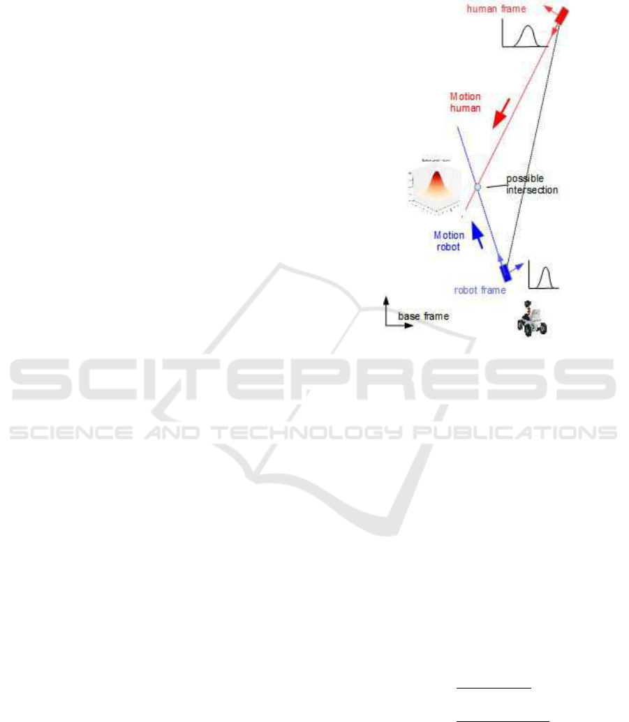
2.1 Computation of Intersections -

Analytical Approach

The following computation deals with the intersection

) of two linear paths x

(t) and x

(t) in a plane

along which robot and human intend to move. x

) and x

= (x

) are the position of human

and robot and φ

and φ

their orientation angles (see

Figs. 1 and 2).

Figure 1: Human-robot scenario.

Then we have the relations

= x

+ d

cos(φ

+ δ

)

= y

+ d

sin(φ

+ δ

) (1)

= x

+ d

cos(φ

+ δ

)

= y

+ d

sin(φ

+ δ

)

where positive angles δ

and δ

are measured from

the y coordinates counterclockwise. Angle

β = π −

−δ

is the angle at the intersection.

The variables x

, x

, φ

, δ

, d

and the an-

gle γ are supposed to be measurable. The unknown

orientation angle φ

is computed by

= arcsin((y

−y

)/d

) −δ

+ π (2)

After some substitutions we obtain the coordinates

and y

straight forward

A −B

tanφ

−tan φ

Atanφ

−B tan φ

tanφ

−tan φ

(3)

A = x

tanφ

−y

B = x

tanφ

−y

Rewriting (3) leads to

Uncertainty and Fuzzy Modeling in Human-robot Navigation

297

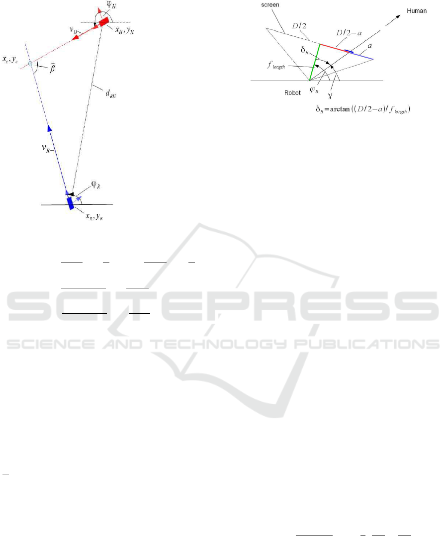
Figure 2: Human-robot scenario: geometry.



tanφ

−y



−



tanφ

−y





tanφ

−y

tanφ



−



tanφ

−y

tanφ



(4)

G = tanφ

−tan φ

which is a form that can be used for the fuzziﬁcation

of (3)

Having a look at (4) we see that x

= (x

)

linear in x

= (x

)

= A

·x

(5)

where

= f (φ

,φ

) =



tanφ

−1 −tanφ

tanφ

−tanφ

tanφ



To achieve the orientation of the human operator

a scenario is recorded by human eye tracking plus a

corresponding camera picture that is taken from the

human’s position and sent to the robot (Palm and

Lilienthal, 2018). The robot measures its own posi-

tion/orientation and the human’s position. From the

human’s screen-shot the robot calculates

- orientation of human

- expected intersection

- direction of human’s gaze to robot or object

- position of object

Figure 3: Camera geometry.

From the robot’s point of view a picture from the

scene is taken from which we obtain a projection of

the human image onto the camera screen(see Fig. 3).

From the focal length f

length

, the width D of the screen

and the distance a, an angle δ

is computed

= arctan((D/2 −a)/ f

length

) (6)

from which the orientation angle φ

of the human is

calculated (see also Fig. 2) and (2)

The TS-fuzzy approximation of (5) is given by

(Palm and Lilienthal, 2018)

∑

i, j

(φ

) ·A

i, j

·x

(7)

(φ

),w

(φ

) ∈ [0,1] are normalized member-

ship functions with

∑

(φ

) = 1 and

∑

(φ

) = 1.

The following paragraph deals with the accuracy of

the computed intersection in the case of distorted ori-

entation information.

2.2 Transformation of Gaussian

Distributions

2.2.1 General Considerations

Let us consider a static nonlinear system

z = F(x) (8)

with two inputs x = (x

)

and two outputs

z = (z

)

where F denotes a nonlinear system. Let

further the uncorrelated Gaussian distributed inputs x

and x

be described by the 2-dim density

2πσ

exp(−

(

)) (9)

where e

= x

− ¯x

, ¯x

- mean(x

), σ

- standard

deviation x

and e

= x

− ¯x

, ¯x

- mean(x

), σ

standard deviation x

The question arises how the output signals z

and

are distributed in order to obtain their standard de-

viations and the correlation coefﬁcient between the

FCTA 2019 - 11th International Conference on Fuzzy Computation Theory and Applications

298

outputs. For linear systems Gaussian distributions are

linearly transformed which means that the output sig-

nals are also Gaussian distributed. In general, this

does not apply for nonlinear system as in our case.

However, if we assume the input standard deviations

small enough then we can construct local linear trans-

fer functions for which the output distributions are

Gaussian distributed but with correlated output com-

ponents.

2πσ

1 −ρ

· (10)

exp(−

2(1 −ρ

)

(

−

2ρ

))

- correlation coefﬁcient.

2.2.2 Differential Approach

Function F can be described by individual smooth and

nonlinear static transfer functions (see block scheme

4) where (x

) = (φ

,φ

) and (z

) = (x

)

= f

)

= f

) (11)

Linearization of (11) yields

dz =

J ·dx or e

J ·e

(12)

with

= (e

)

and e

= (e

)

(13)

dz = (dz

,dz

)

and dx = (dx

,dx

)

J =



∂ f

/∂x

,∂ f

/∂x

∂ f

/∂x

,∂ f

/∂x



(14)

Figure 4: Differential transformation.

2.2.3 Speciﬁc Approach to the Intersection

In addition to the exact solution (4) we look at the

differential approach. This is important if the con-

tributing agents change their directions of motion. A

further aspect is to quantify the uncertainty of x

the presence uncertain angles φ

and φ

or in x

)

Differentiating (4) with x

= const. yields

J ·

φ = (

)

;

J =





(15)

where



−tanφ

1 tanφ

−1



·cos



tanφ

−1 −tanφ



·cos

·tan φ

2.2.4 Output Distribution

To obtain the density f

of the output signal we

invert (13) and substitute the entries of e

into (9)

= J ·e

(16)

with J =

−1

and

J =









(17)

where j

= (J

) and j

= (J

). Entries J

i j

are the result of the inversion of

J. From this substi-

tution which we get

= K

exp(−

·e

·(j

) ·S

−1





·e

) (18)

where K

2πσ

and

−1









(19)

The exponent of (18) is rewritten into

xpo = −

·(

+ e

)

+ e

)

) (20)

and furthermore

xpo = −

·[e

(

) + e

(

) +

2 ·e

(

)] (21)

Uncertainty and Fuzzy Modeling in Human-robot Navigation

299

Now, we compare xpo in (21) with the exponent

in (10) of the output density (10)

Let

A = (

); B = (

)

C = (

) (22)

then a comparison of xpo in (21) and the exponent in

(10) yields

(1 −ρ

)

= A;

(1 −ρ

)

= B

−2ρ

(1 −ρ

)

= 2C (23)

from which we ﬁnally get the correlation coefﬁcient

and the standard deviations σ

and σ

= −

√

= A −

;

= B −

(24)

So once we have obtained the parameters of the

input distribution and the mathematical expression for

the transfer function F(x,y) we can compute the out-

put distribution parameters directly.

3 INVERSE SOLUTION

In the previous presentation we discussed the prob-

lem: Given the parameters of the input distributions

of a nonlinear system, ﬁnd the parameters of the out-

put distributions. In a bearing task that runs from dif-

ferent positions for the same target it might be helpful

to deﬁne a particular bearing accuracy while ﬁnding

out the necessary accuracy of the bearing instruments

with regard their bearing angles.

This inverse task we apply is similar to that we dis-

cussed in section 2.2.2. The starting point is equation

(13). Equations (10) describe the densities of the in-

puts and the outputs, respectively. Then we substitute

(13) into (10) and discuss the exponent xpo

only

xpo

−1

2(1 −ρ

)

−1

−

2ρ

) (25)

where

−1









(26)

With

= (

) ·(

);

−1

(

) + e

(

)

+2e

(

) (27)

we obtain for the exponent xpo

xpo

= −

2(1 −ρ

)

(

) +

(

) + 2e

(

) −

2ρ

(

) ·(

)) (28)

and further

xpo

= −

(

−

2ρ

)/(1 −ρ

)

(

−

2ρ

)/(1 −ρ

)

(1 −ρ

)

·(

−

(

)))

(29)

Now, comparing (29) with the exponent of (10) of

the input density we ﬁnd that the mixed term in (29)

should be zero from which we obtain the correlation

coefﬁcient and the standard deviations of the inputs

= (

)

(

)

(30)

= (

−

2ρ

)/(1 −ρ

) (31)

= (

−

2ρ

)/(1 −ρ

) (32)

4 FUZZY SOLUTION

The previous presentation shows that the computa-

tion of the output distribution can be associated with

high costs which might be problematic especially in

the on-line case. Provided that an analytical represen-

tation (8) is available then we can build a TS fuzzy

model by the following rules R

i j

FCTA 2019 - 11th International Conference on Fuzzy Computation Theory and Applications

300

i j

: (33)

IF x

= X

AND x

= X

T HEN ρ

= −

i j

AND

= A

i j

−

i j

;

AND

= B

i j

−

i j

where X

are fuzzy terms for x

, A

i j

are functions of predeﬁned variables x

= x

and x

From (33) we get

= −

∑

i j

)

i j

∑

i j

)(A

i j

−

i j

) (34)

∑

i j

)(B

i j

−

i j

)

) ∈ [0, 1] and w

) ∈ [0, 1] are weighting

functions with

∑

) = 1

∑

) = 1

5 EXTENSION TO SIX INPUTS

AND TWO OUTPUTS

The previous section dealt with two orientation inputs

and two intersection position outputs where the posi-

tion coordinates of robot and human are assumed to

be constant. Let us again consider the nonlinear sys-

tem

= F(x) (35)

where F denotes a nonlinear system. Here we

have 6 inputs x = (x

)

and 2 out-

puts x

= (x

)

. For the bearing problem we get

x = (φ

,φ

)

Let further the uncorrelated Gaussian distributed

inputs x

... x

be described by the 6-dim density

(2π)

6/2

1/2

exp(−

−1

)) (36)

where e

= (e

,...,e

)

; e

= x−

x - mean(x),

- covariance matrix.







0 ... 0

0 σ

... 0

... ... ... ...

0 ... 0 σ







The output density is again described by

2πσ

1 −ρ

· (37)

exp(−

2(1 −ρ

)

−1

−

2ρe

))

ρ - correlation coefﬁcient.

In correspondence to (8) and (11) function F can

be described by

= f

(x) (38)

= f

(x)

Furthermore we have in correspondence to (15)

J ·e

(39)

with

J =



...



(40)

where

i j

∂ f

∂x

, , i = 1, 2 , j = 1,...,6 (41)

Inversion of (40) leads to

·e

= J ·e

(42)

with the pseudo inverse

= J of

J =





... ...





(43)

where

−1

(44)

Substituting (39) into (36) we obtain

= K

exp(−

−1

)) (45)

where K

represents a normalization of the output

density and

Uncertainty and Fuzzy Modeling in Human-robot Navigation

301

= J

−1

J =



A B

C D



where

A =

∑

i=1

; B =

∑

i=1

(46)

C =

∑

i=1

; D =

∑

i=1

Substitution of (46) into (45) leads with B = C to

= K

exp(−

(Ae

+ De

+ 2Ce

)) (47)

Comparison of (47) with (37) leads with (44) to

ρ = −

√

= A −

;

= D −

(48)

which is the counterpart to the 2 dim input case (24).

5.1 Fuzzy Approach

The ﬁrst step is to compute values A

, B

and C

from (46) at predeﬁned positions/orientations x =

)

. Then, we formulate fuzzy rules

, according to (33) and (34) with i = 1...n, l - num-

ber of fuzzy terms, k = 6 - number of variables n = l

- number of rules. With such an increase in the num-

ber of inputs, one unfortunately sees the problem of

an exponential increase in the number of rules, which

is associated with a very high computational burden.

For l = 7 fuzzy terms for each input variable x

k = 6 we end up with n = 7

rules which is much

to high to deal with in a reasonable way. So, one

has to restrict to a reasonable number of variables at

the input of a fuzzy system. This can be done ei-

ther in a heuristic or systematic way (J.Schaefer and

K.Strimmer, 2005) to ﬁnd out the most inﬂuential in-

put variables which is however not the issue of this

paper.

6 MIXED GAUSSIAN

DISTRIBUTIONS

For input signals with larger standard deviations one

cannot assume that the fuzzy system is almost linear

within the operating area. For this reason a distribu-

tion with large standard deviation is approximated by

several distributions with small standard deviations,

where the linearization of the fuzzy system around

their mean values applies. The following analysis ap-

plies with the analytical approach and the fuzzy ap-

proximation too. Let us concentrate on an example of

a mixture of two distributions/densities f

xy1

and f

xy2

xy1

2πσ

exp(−

(

)) (49)

xy2

2πσ

exp(−

(

)) (50)

that are linearly combined

= a

xy1

+ a

xy2

(51)

with a

>= 0 and

∑

= 1 where i = 1, 2

and

= x

− ¯x

; e

= x

− ¯x

= y

− ¯y

; e

= y

− ¯y

¯x

, ¯y

are the mean values of x

The partial outputs yield

2πσ

1 −ρ

· (52)

exp(−

2(1 −ρ

)

(

−

2ρ

))

= z

−¯z

; e

= z

−¯z

; ρ

- correlation coefﬁcient.

From this we ﬁnally obtain the output distribution

∑

i=1

(53)

The mixed output distribution f

is a linear com-

bination of partial output distributions f

as a re-

sult of the input distributions f

x,y

. Given the mean

¯z

,k = 1,2 and variance σ

of the partial output dis-

tributions f

. Then we ﬁnd for mean and variance

of the mixed output distribution

¯z

∑

i=1

¯z

(54)

= a

(σ

)

+ a

(σ

)

+ a

(¯z

− ¯z

)

from which we obtain the standard deviation σ

of the intersection straight forward.

FCTA 2019 - 11th International Conference on Fuzzy Computation Theory and Applications

302

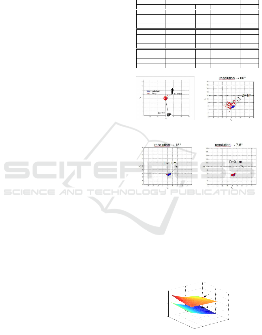
7 SIMULATION RESULTS

Gaussian Input Distributions.

Based on the human-robot intersection example, the

following simulation results show the feasibility to

predict uncertainties at possible intersections by us-

ing analytical and/or fuzzy models for a static situa-

tion (see ﬁg. 2)). Position/orientation of robot and

human are given by x

= (x

) = (2,0)m and x

) = (4,10)m and φ

= 1.78 rad, (= 102

◦

), and

= 3.69 rad, (= 212

◦

). φ

and φ

are corrupted

with Gaussian noise with standard deviations (std)

of σ

= σ

= 0.02 rad, (= 1.1

◦

). We compared

the fuzzy approach with the analytical non-fuzzy ap-

proach using partitions of 60

◦

,30

◦

,15

◦

,7.5

◦

of the

unit circle for the orientations with results shown in

table 1 and ﬁgures 5-8. Notations in table 1 are: σ

- std-computed, σ

- std-measured etc. The num-

bers show two general results:

1. Higher resolutions lead to better results.

2. The performance regarding measured and com-

puted values depends on the shape of membership

functions (mf’s). Lower input std’s (0.02 rad) require

Gaussian mf’s, higher input std’s (0.05 rad = 2.9

◦

)

require Gaussian bell shape mf’s which can be ex-

plained by different smoothing effects (see columns 4

and 5 in table 1).

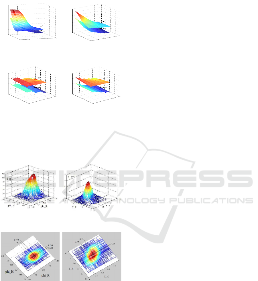
Results 1 and 2 can be explained by the comparison of

the corresponding control surfaces and the measure-

ments (black and red dots) to be seen in ﬁgures 9 -

13. Figure 9 displays the control surfaces of x

and y

for the analytical case (4). The control surfaces of the

fuzzy approximations (7) (see (Palm and Lilienthal,

2018)) are depicted in ﬁgures 10 - 13. Starting from

the resolution 60

◦

(ﬁg. 10) we see a very high devia-

tion compared to the analytic approach (ﬁg. 9) which

decreases more and more down to resolution 7.5

◦

(ﬁg.

13). This explains the high deviations in standard de-

viations and correlation coefﬁcients in particular for

sector sizes 60

◦

and 30

◦

Mixed Gaussian Distributions.

Due to larger uncertainties of the orientations of

robot and human we assume the input signals to

be a mixture of two Gaussian distributions with the

following parameters:

= 1.779 rad,(102 deg), σ

= 0.02 rad

= 3.698 rad,(212 deg), σ

= 0.02 rad

= 1.762 rad,(101 deg), σ

= 0.03 rad

= 3.716 rad,(213 deg), σ

= 0.03 rad

= 0.1309 rad; σ

= 0.1157 rad

= 0.2274 rad; σ

= 0.1978 rad

Table 1: Standard deviations, fuzzy and non-fuzzy results.

input std 0.02 Gauss, bell shaped (GB) Gauss 0.05 GB

sector size/

◦

7.5

◦

7.5

◦

7.5

◦

non-fuzz σ

0.143 0.140 0.138 0.125 0.144 0.366

fuzz σ

0.220 0.184 0.140 0.126 0.144 0.367

non-fuzz σ

0.160 0.144 0.138 0.126 0.142 0.368

fuzz σ

0.555 0.224 0.061 0.225 0.164 0.381

non-fuzz σ

0.128 0.132 0.123 0.114 0.124 0.303

fuzz σ

0.092 0.087 0.120 0.112 0.122 0.299

non-fuzz σ

0.134 0.120 0.123 0.113 0.129 0.310

fuzz σ

0.599 0.171 0.034 0.154 0.139 0.325

non-fuzz ρ

0.576 0.541 0.588 0.561 0.623 0.669

fuzz ρ

-0.263 0.272 0.478 0.506 0.592 0.592

non-fuzz ρ

0.572 0.459 0.586 0.549 0.660 0.667

fuzz ρ

0.380 0.575 0.990 0.711 0.635 0.592

Figure 5: Sector size: 60

deg.

Figure 6: Sector size: 30

deg.

Figure 7: Sector size: 15

deg.

Figure 8: Sector size: 7.5

deg.

The following computed non-fuzzy and fuzzy (su-

perscript F) and measured numbers (superscript m)

according to (54) show the correctness of the previ-

ous analysis for the analytical case.

¯z

= 0.487; ¯z

= 0.413; ¯z

= 0.485

¯z

= 7.746; ¯z

= 7.737; ¯z

= 7.737

= 0.222; σ

= 0.235; σ

= 0.199

= 0.184; σ

= 0.178

1.2

1.4

1.6

1.8

3.2

3.4

3.6

3.8

−5

phi

Figure 9: Control surface non-fuzzy.

Uncertainty and Fuzzy Modeling in Human-robot Navigation

303

1.2

1.4

1.6

1.8

3.5

−20

100

phi

Figure 10: Control surface

fuzzy, 60

◦

1.2

1.4

1.6

1.8

3.2

3.4

3.6

3.8

−5

phi

Figure 11: Control surface

fuzzy, 30

◦

1.2

1.4

1.6

1.8

3.2

3.4

3.6

3.8

−5

phi

Figure 12: Control surface

fuzzy, 15

◦

1.2

1.4

1.6

1.8

3.2

3.4

3.6

3.8

−5

phi

Figure 13: Control surface

fuzzy, 7.5

◦

Figures 14 and 15 show the regarding input and

output densities where Figs. 16 and 17 depict the scat-

ter diagrams (cuts at certain density levels). Finally it

turns out that the fuzzy approximation is sufﬁciently

accurate.

Figure 14: Mixed Gaussian,

input.

Figure 15: Mixed Gaussian,

output.

Figure 16: Scatter diagram,

mixed input.

Figure 17: Scatter diagram,

mixed output.

8 CONCLUSIONS

The work presented in this paper is motivated by the

task to predict future situations such as collisions at

speciﬁc areas in the presence of robots and humans

and to use this information for feed forward control

actions in the presence of uncertainties. This is essen-

tial for human intentions, actions and reactions that

are difﬁcult to predict and interpret by a robot. We

discussed the problem of intersections of trajectories

in human-robot systems with respect to uncertainties

that are modeled by Gaussian noise on the orienta-

tions of human and robot. This problem is solved by

a transformation from human-robot orientations to in-

tersection coordinates using a geometrical model and

its TS fuzzy version. Based on the input standard de-

viations of the orientations of human and robot, the

output standard deviations of the intersection coordi-

nates are calculated. The analysis was performed un-

der the condition that the nominal position/orientation

of robot and human are constant and known. The

measurements of their orientations are distorted by

Gaussian noise with known parameters. This analy-

sis together with the fuzzy extension also applies to

robots and humans in motion, as long as the positions

of robots and humans can be reliably estimated. We

also extended our method to six inputs and two out-

puts which includes human/robot positions as well.

For the analytical and the fuzzy version of two-input

case the following inverse task can also be solved:

given the standard deviation for the intersection co-

ordinates, ﬁnd the corresponding input standard devi-

ations for the orientations of robot and human. For

larger standard deviations of the orientation signals

the method is ﬁnally extended to mixed Gaussian dis-

tributions. In summary, predicting the accuracy of

human-robot cooperation at a small distance using the

methods presented in this paper increases the system

performance and human safety of human-robot col-

laboration. In future work this method will be used

for robot-human scenarios in factory workshops and

for robots working in difﬁcult environments like res-

cue robots in cooperation with human operators.

ACKNOWLEDGMENT

This research work has been supported by the AIR-

project, Action and Intention Recognition in Human

Interaction with Autonomous Systems.

REFERENCES

Banelli, P. (2013). Non-linear transformations of gaussians

and gaussian-mixtures with implications on estima-

tion and information theory. IEEE Trans. on Infor-

mation Theory.

Bruce, J., Wawer, J., and Vaughan, R. (2015). Human-robot

rendezvous by co-operative trajectory signals. pages

1–2.

Firl, J. (2014). Probabilistic maneuver recognition in trafﬁc

scenarios. Doctoral dissertation, KIT Karlsruhe,.

FCTA 2019 - 11th International Conference on Fuzzy Computation Theory and Applications

304

Fraichard, T., Paulin, R., and Reignier, P. (2014). Human-

robot motion: Taking attention into account . Re-

search Report, RR-8487.

H.Hellendoorn and R.Palm (1994). Fuzzy system technolo-

gies at siemens r and d. Fuzzy Sets and Systens 63

(3),1994, pages 245–259.

J.Chen, Wang, C., and Chou, C. (2018). Multiple tar-

get tracking in occlusion area with interacting ob-

ject models in urban environments. Robotics and Au-

tonomous Systems, Volume 103, May 2018, pages 68–

82.

J.Schaefer and K.Strimmer (2005). A shrinkage to large

scale covariance matrix estimation and implications

for functional genomics. Statistical Applications in

Genetics and molecular Biology, vol. 4, iss. 1, Art. 32.

Kassner, M., W.Patera, and Bulling, A. (2014). Pupil: an

open source platform for pervasive eye tracking and

mobile gaze-based interaction. In Proceedings of the

2014 ACM international joint conference on pervasive

and ubiquitous computing, pages 1151—1160. ACM.

Khatib, O. (1985). Real-time 0bstacle avoidance for ma-

nipulators and mobile robots. IEEE Int. Conf. On

Robotics and Automation,St. Loius,Missouri, 1985,

page 500-505.

L.Foulloy and S.Galichet (2003). Fuzzy control with fuzzy

inputs. IEEE Trans. Fuzzy Systems, 11 (4), pages 437–

449.

O.H.Hamid and N.L.Smith (2017). Automation, per se, is

not job elimination: How artiﬁcial intelligence for-

wards cooperative human-machine coexistence. In

Proceedings IEEE 15th International Conference on

Industrial Informatics (INDIN), pages 899–904, Em-

den, Germany. IEEE.

Palm, R., Chadalavada, R., and Lilienthal, A. (2016).

Fuzzy modeling and control for intention recognition

in human-robot systems. In 7. IJCCI (FCTA) 2016:

Porto, Portugal.

Palm, R. and Iliev, B. (2006). Learning of grasp behaviors

for an artiﬁcial hand by time clustering and takagi-

sugeno modeling. In Proceedings FUZZ-IEEE 2006

- IEEE International Conference on Fuzzy Systems,

Vancouver, BC, Canada. IEEE.

Palm, R. and Iliev, B. (2007). Segmentation and recognition

of human grasps for programming-by-demonstration

using time clustering and takagi-sugeno modeling. In

Proceedings FUZZ-IEEE 2007 - IEEE International

Conference on Fuzzy Systems, London, UK. IEEE.

Palm, R. and Lilienthal, A. (2018). Fuzzy logic and control

in human-robot systems: geometrical and kinematic

considerations. In WCCI 2018: 2018 IEEE Inter-

national Conference on Fuzzy Systems (FUZZ-IEEE),

pages 827–834. IEEE, IEEE.

Pota, M., M.Esposito, and Pietro, G. D. (2011). Trans-

formation of probability distribution into a fuzzy set

interpretable with likelihood view. In IEEE 11th In-

ternational Conf. on Hybrid Intelligent Systems (HIS

2011), pages 91–96, Malacca Malaysia. IEEE.

Robertsson, L., Iliev, B., Palm, R., and Wide, P. (2007).

Perception modeling for human-like artiﬁcial sensor

systems. International Journal of Human-Computer

Studies 65 (5), pages 446–459.

R.Palm and Driankov, D. (1993). Tuning of scaling fac-

tors in fuzzy controllers using correlation functions.

In Proceedings FUZZ-IEEE’93, San Francisco, cali-

fornia. IEEE, IEEE.

R.Palm and Driankov, D. (1994). Fuzzy inputs. Fuzzy Sets

and Systems - Special issue on modern fuzzy control,

pages 315–335.

Tahboub, K. A. (2006). Intelligent human-machine interac-

tion based on dynamic bayesian networks probabilis-

tic intention recognition. Journal of Intelligent and

Robotic Systems., Volume 45, Issue 1:31–52.

W.Luo, J.Xing, Milan, A., Zhang, X., Liu, W., Zhao, X.,

and Kim, T. (2014). Multiple object tracking: A liter-

ature review. Computer Vision and Pattern Recogni-

tion, arXiv 1409,7618, page 1-18.

Yager, R. and Filev, D. B. (1994). Reasoning with proba-

bilistic inputs. In Proceedings of the Joint Conference

of NAFIPS, IFIS and NASA, pages 352–356, San An-

tonio. NAFIPS.

Uncertainty and Fuzzy Modeling in Human-robot Navigation

305