Fireworks Algorithm versus Plant Propagation Algorithm
Wouter Vrielink
1
and Daan van den Berg
2
1
Computational Science Lab., Universiteit van Amsterdam, Science Park 904, Amsterdam, The Netherlands
2
Institute for Informatics, Universiteit van Amsterdam, Science Park 904, Amsterdam, The Netherlands
Keywords:
Plant Propagation Algorithm, Fireworks Algorithm, Evolutionary Algorithm, Optimization Algorithm,
Comparison, Metaheuristics.
Abstract:
In recent years, the field of Evolutionary Algorithms has seen a tremendous increase in novel methods. While
these algorithmic innovations often show excellent results on relatively limited domains, they are less often
rigorously cross-tested or compared to other state-of-the-art developments. Two of these methods, quite similar
in their appearance, are the Fireworks Algorithm and Plant Propagation Algorithm.
This study compares the similarities and differences between these two algorithms, from both quantitative and
qualitative perspectives, by comparing them on a set of carefully chosen benchmark functions. The Fireworks
Algorithm outperforms the Plant Propagation Algorithm on the majority of these, but when the functions
are shifted slightly, Plant Propagation gives better results. Reasons behind these surprising differences are
presented, and comparison methods for evolutionary algorithms are discussed in a wider context. All source
code, graphs, test functions, and algorithmic implementations have been made publicly available for reference
and further reuse.
1 INTRODUCTION
The increasingly popular field of population-based
metaheuristics aims to create assumption-free and flex-
ible algorithms. These Population-Based Algorithms
(PBA) are transferable to different problem domains,
easily implemented, almost effortlessly combined with
exact methods, and capable of finding multiple solu-
tions in a single run. Essential in the development
of optimization algorithms is to balance exploration
and exploitation. Exploration refers to the ability to
sample the entire problem domain, ensuring that mul-
tiple options are considered. Exploitation refers to the
ability to converge to a local optimum once in its basin,
which is reflected directly in the quality of the solution
found by the algorithm. It is important to correctly
balance these properties to prevent getting stuck in
local optima, or from never finding a neighbouring
solution that might be better (Alba and Dorronsoro,
2005; Audibert et al., 2009; Ishii et al., 2002).
The Fireworks Algorithm (FWA) (Tan and Zhu,
2010) and the Plant Propagation Algorithm (PPA)
(Salhi and Fraga, 2011) share a lot of algorithmic sim-
ilarities and experimental results. Both are population-
based algorithms that rely on normalizing fitness val-
ues of the individuals to (0, 1) . In both algorithms,
relatively fit individuals generate many offspring with
small mutations, whereas relatively unfit individuals
generate few offspring with large mutations. As such –
even though the procedural details differ – both algo-
rithms attempt to balance exploration and exploitation
through relating the number of offspring and the de-
gree of mutation to the normalized fitness of its par-
ents.
Both FWA and PPA normalize fitness values; the
best individual within the current population has a
fitness of 1 , whereas the worst individual within the
current population has a fitness of 0 . This makes the
algorithms insensitive to linear changes or translations
of the range of the objective function, as the relative
difference between individuals does not depend on
this range. The number of algorithmic parameters is
reduced and less domain-specific assumptions have to
be made, which in turn reduces the knowledge required
about the algorithm and the effort required to find
optimal algorithmic parameters.
The principle of reducing the number of algorith-
mic parameters can also be identified in the procedure
that is responsible for the generation of offspring. In
both algorithms, offspring are generated from a sin-
gle parent. This eliminates the need for a crossover
method, which – depending on the method used or
the problem the algorithm is applied to – could be a
source of constraint violation, requiring subsequent
Vrielink, W. and van den Berg, D.
Fireworks Algorithm versus Plant Propagation Algorithm.
DOI: 10.5220/0008169401010112
In Proceedings of the 11th International Joint Conference on Computational Intelligence (IJCCI 2019), pages 101-112
ISBN: 978-989-758-384-1
Copyright
c
 2019 by SCITEPRESS – Science and Technology Publications, Lda. All rights reserved
101

repair methods and adding unnecessary complexity.
However, this could be at the expense of combining
good properties from multiple individuals into one and
therefore could reduce exploitative properties of the
algorithms (Paauw and van den Berg, 2019). Nonethe-
less, these principles create algorithms that are more
widely applicable, as is so aptly described by Kenneth
S
¨
orensen (S
¨
orensen, 2015). Many “novel” methods
seem unnecessarily complex, are rarely extensively
tested, or may introduce undesirable biases (S
¨
orensen,
2015; Weyland, 2015).
Today, a quantitative comparison and qualitative
treatise on the differences and similarities between
the Fireworks Algorithm and the Plant Propagation
Algorithm is presented. Strengths and weaknesses of
both algorithms will be uncovered and performance
analyses will be made to understand exactly how these
algorithms differ and to what extent methods can be
used to reduce the number of meta-parameters while
increasing performance.
1.1 Related Work
Population-based algorithms are proving to be very
successful in complex optimization problems and can
occasionally overcome the drawbacks of traditional
mathematical methods. The primary feature of PBA’s
is that, unlike heuristic methods such as Simulated
Annealing (SA) (Kirkpatrick et al., 1983) and Tabu
Search (TS) (Glover, 1989, 1990), evaluation of many
candidate solutions is done simultaneously. The con-
current evaluation of many solutions enables the ex-
ploration of the search-space utilizing the collective
intelligence that arises from these solutions, potentially
avoiding local minima.
A classic success story of a Genetic Algorithm
(GA) is that of reducing vibrations (and weight) of a
space satellite boom structure (Moshrefi-Torbati et al.,
2003; Keane, 1996). The GA significantly improved
an existing design to 30 dB of energy transmission
isolation between both ends. It has even actually been
built. However, the evaluation procedure for this multi-
objective optimization problem comes with great com-
putational costs (El-Beltagy and Keane, 2001).
One older example of a variant of a PBA that is
still often referred to is Differential Evolution (DE)
(Storn and Price, 1997). The algorithm was developed
with four main requirements in mind: the ability to
handle different types of objective functions, paral-
lelizability, ease of use (through a small number of
control variables that are easy to choose), and consis-
tent convergence properties. The main principle of
DE is to adding the weighted difference between two
objective function’s parameter vectors to a randomly
chosen third vector. This algorithm is very simple to
implement and at the time of publishing (1997) outper-
formed many of the then prevalent strategies.
Another nature-inspired heuristic optimization al-
gorithm that is often used in comparisons of opti-
mization algorithms is the Harmony Search Algorithm
(HSA) (Geem et al., 2001). It attempts to mimic the
improvisation of musicians by evolving what it calls
a set of “harmonies” that in turn consist of “pitches”
1
. The main difference between HSA and GA is that
HSA considers more than two parents when gener-
ating offspring and that it requires no careful choice
of initial values. HSA shows good results for both
discrete and continuous optimization problems, but is
also criticized for not offering any novelty, apart from
using a different terminology (Weyland, 2015).
The algorithms discussed in this study (FWA (Tan
and Zhu, 2010) and PPA (Salhi and Fraga, 2011)) were
published within such a narrow timeframe that the
submissions might have easily crossed one another.
However, FWA seems to be much more popular in the
community than PPA. At the time of writing, more
than 50 papers with “Fireworks Algorithm” in the
title are available on Google Scholar, at least 10 of
which have more than 50 citations. PPA has around
ten papers with “Plant Propagation Algorithm” in their
titles on Google Scholar, which have also been cited
less often. A rough estimate would be that FWA is
around five times bigger, in numbers of papers, in
numbers of citations and possibly in the number of
involved researchers.
The paper by Imran and Kowsalya (2014) is an
interesting example of a real-world optimization prob-
lem that is solved by applying FWA. It shows a method
using FWA to solve the problem of power system net-
work reconfiguration in such a way that power loss
and voltage profile is minimized. In this paper, FWA is
compared with other classical methods from literature
(GA, Refined GA, Improved TS, and HSA) and it is
shown that FWA outperforms these methods in general
quality of solutions.
Likewise, a recent example of PPA being applied to
several real-world constrained optimization problems
can be found in Sulaiman et al. (2014b). Herein PPA is
found to be as good, or in some cases superior to, state-
of-the-art optimization algorithms. More recently, a
discrete version of PPA has been shown to perform
admirably on the Traveling Salesman Problem (TSP),
where it outperformed GA and SA both in solution
quality and in runtime (Selamo
˘
glu and Salhi, 2016).
Interestingly, like S
¨
orensen’s paper, this paper also
1
Harmonies can be interpreted as individuals, while
pitches can be interpreted as distinct discrete values of one
parameter inside its domain.
ECTA 2019 - 11th International Conference on Evolutionary Computation Theory and Applications
102

poses the idea of comparing algorithms or heuristics
on a number of other criteria than just performance;
“[the criterion consisting of the number of arbitrarily
set parameters required by a given heuristic algorithm
is interesting because it does not depend on the pro-
gramming skills of the researcher, the quality of code,
the language of coding, the compiler or the processor.
It is intrinsic to the algorithm itself.]” (Selamo
˘
glu and
Salhi, 2016).
Finally, in Cheraitia et al. (2017), a hybrid ver-
sion of PPA and Local Search (LS) is used to solve
the uncapacitated exam scheduling problem (UESP).
Similarly, Geleijn et al. (2019) presents a non-hybrid
version of PPA to solve the UESP. The UESP is a
well-known computationally intractable combinatorial
optimization problem that aims to schedule exams to
periods while avoiding conflicts and spreading exams
as evenly as possible. The papers show good results
and demonstrate that PPA can easily be adapted to
different types of problems.
1.2 Adaptations in Later Papers
EFWA (Enhanced FWA), as presented in Zheng et al.
(2013), proposes five improvements over FWA: a new
minimal explosion amplitude, a new method of gen-
erating explosion sparks, a new mapping strategy for
sparks which are out of bounds, a new operator for
generating Gaussian sparks and a new method for se-
lection of individuals. EFWA not only outperforms
FWA in convergence, but it also reduces runtime sig-
nificantly (Zheng et al., 2013).
An adaptive approach (AFWA) is proposed for
EFWA, wherein the formulas that determine the mag-
nitude of mutation with which a new individual is
generated are replaced with adaptive versions (Li et al.,
2014). In this study, the distance at which new indi-
viduals are generated depends on information gained
during the last iteration. The selected distance is pro-
portional to the distance between the best new off-
spring and the closest offspring that is worse than the
parent, as this is the area that will most likely hold bet-
ter results. This results in performance improvement
over EFWA, while it does not significantly increase
computational costs.
Similarly, a dynamic approach (DynFWA) is pro-
posed wherein an attempt is made to speed up conver-
gence by increasing or decreasing the mutability of
offspring proportional to the increase in fitness from
the last iteration (Zheng et al., 2014). If the current
best individual increases in fitness during an iteration,
the mutability of the next generation is increased. Con-
versely, when the fitness does not increase, the mu-
tability of new individuals is decreased. Offspring
generated by other parents are generated according to
earlier EFWA-methods. Furthermore, the study argues
that Gaussian sparks can be removed from the algo-
rithm entirely, as in most results they will not increase
diversity. Again, this results in equal or sometimes bet-
ter performance than EFWA while reducing runtime.
Likewise, a variant of the original algorithm has
been designed for PPA; a variant named MPPA (Mod-
ified PPA), as presented in Sulaiman et al. (2014a).
MPPA uses a fixed number of offspring instead of us-
ing the relative fitness of an individual to calculate
its number of offspring. Furthermore, new individu-
als are generated one by one, where if it is not better
than its parent, it is discarded and a new individual
is generated. This is repeated up to three times, each
time using a different formula when generating the
position of the new individual. MPPA shows better
performance than PPA and the Artificial Bee Colony
Algorithm (Sulaiman et al., 2014a).
Although there are many published adaptations on
the original algorithms, the comparison in this study is
made between the original descriptions of FWA and
PPA only. Both algorithms are implemented from
scratch and have their performance compared on a
specific set of benchmark test functions. But first, the
algorithms will be functionally aligned for qualitative
comparison.
2 FIREWORKS & PLANT
PROPAGATION
Although FWA and PPA abide by very similar algorith-
mic philosophies, equations and routines are deployed
differently. A perfect example of this can be found
in the order of procedures which are common for all
population-based algorithms: initialization, offspring
generation, and selection of individuals. FWA starts
with initialization, then loops over generating offspring
and selecting individuals respectively. PPA also starts
with initialization, but then loops over selecting indi-
viduals and generating offspring. Although the order
of these procedures is different for FWA and PPA, they
can be interchanged without loss of generality. For
a uniformly formatted overview of both algorithms,
the reader is referred to table 1. In order to facilitate
comparison and ease of reading the formulas and ter-
minology are linguistically generalized, but otherwise
stay functionally consistent with the seminal papers
(Tan and Zhu, 2010; Salhi and Fraga, 2011).
Initialization of the population
, as done in the
seminal papers (Tan and Zhu, 2010; Salhi and Fraga,
2011), is nearly identical for FWA and PPA. Individu-
als in the initial population are generated by drawing
Fireworks Algorithm versus Plant Propagation Algorithm
103

Table 1: Algorithmic subroutines of FWA and PPA where N represents the size of the current population, x
max
and x
min
the
current best and worst individual, r ∈ [0, 1) a uniform random number, x
i j
the position of individual i in dimension j , the
benchmark function f , the number of dimensions in the benchmark function D , and a
j
and b
j
the lower and upper bound of the
benchmark function in dimension j . Algorithm specific parameters are: PopSize the number of individuals in a population
after selection, ˆm the parameter that controls the number of offspring per individual, m the parameter that controls the number
of Gaussian Sparks, n
max
and n
min
the maximum and minimum number of offspring per individual, and d
max
the maximum
distance of offspring.
Subroutine FWA PPA
Initialization of the
population
PopSize individuals uniform random over whole domain
PopSize individuals uniform random
over whole domain
Assigning fitness
F
1
(x
i
) =
f (x
max
)−f (x
i
)+ε
∑
N
i=1
( f (x
max
)−f (x
i
))+ε
F
2
(x
i
) =
f (x
i
)−f (x
min
)+ε
∑
N
i=1
( f (x
i
)−f (x
min
))+ε
z(x
i
) =
f (x
max
)−f (x
i
)
f (x
max
)−f (x
min
)
F(x
i
) =
1
2
(tanh(4 ·z(x
i
) −2) + 1)
Number of offspring
ˆn(x
i
) = ˆmF
1
(x
i
)
n(x
i
) =





n
min
if ˆn(x
i
) < n
min
n
max
if ˆn(x
i
) > n
max
round(ˆn(x
i
)) otherwise
n(x
i
) = dn
max
F(x
i
)re
Position of offspring
d(x
i
) = 2(r −0.5)F
2
(x
i
)d
max
for dD ·re random dimensions, do: x
∗
i j
= x
i j
+ d(x
i
)
d
j
(x
i
) = 2(r −0.5)(1 −F(x
i
))
x
∗
i j
= x
i j
+ (b
j
−a
j
)d
j
(x
i
)
Generating additional
(Gaussian) offspring
m extra individuals -
Position of additional
(Gaussian) offspring
g = N (µ, σ
2
), with µ = σ = 1
for dD ·re random dimensions, do: x
∗
i j
= x
i j
∗g
-
Bounds correction
x
∗
i j
=
(
x
∗
i j
if a
j
<= x
∗
i j
<= b
j
a
j
+ |x
∗
i j
| mod (b
j
−a
j
) otherwise
x
∗
i j
=





a
j
if x
∗
i j
< a
j
b
j
if x
∗
i j
> b
j
x
∗
i j
otherwise
Selection of individuals
Best individual and PopSize −1 additional individuals
which are selected through:
R(x
i
) =
∑
j∈N
||x
i
−x
j
||
p
selection
(x
i
) =
R(x
i
)
∑
j∈N
R(x
j
)
Best PopSize individuals are selected
a uniform random number from the entire domain for
each of the dimensions. Although in the seminal pa-
per on FWA initialization is done on either [30, 50]
D
or [15, 30]
D
, personal correspondence with the author,
Ying Tan, confirmed that this could just as well be done
on the entire domain, ultimately making it identical to
PPA’s initialization method.
Assigning fitness for both algorithms is done by
‘normalizing’ the fitness values for all individuals in
the population to lie in (0, 1) . One big difference be-
tween FWA and PPA is that FWA defines two differ-
ent formulas for the calculation of relative fitness for
each individual: F
1
(x
i
) and F
2
(x
i
) . The outcome of F
1
increases proportionately from the best to the worst
individual and is used when calculating the number of
offspring that an individual generates. Contrarily, the
outcome of F
2
decreases proportionate from the best
to the worst individual and is used when deciding the
mutation size of the newly generated offspring. To-
gether, the two formulas form the essence of FWA’s
paradigm; good individuals produce many offspring
with small mutations, and bad individuals vice versa.
Although it abides by the same paradigm, PPA de-
fines the normalized or ‘relative’ fitness values with
just one formula: F(x
i
) . The outcome of this formula
is then used to calculate the number of offspring for an
individual, where higher values result in a higher num-
ber of offspring. Conversely, the inverse ( 1 −F(x
i
) )
is proportionate to the mutation size of the offspring.
However, unlike FWA, the relative fitness is calcu-
lated in two steps: the individual’s objective values are
first normalized to be in [0, 1] , after which a ‘mapping
function’ (a hyperbolic tangent) ensures that values
lie strictly in (0, 1) . As the authors note: this is nec-
essary, because the methods that are used to calcu-
late the offspring distance would otherwise produce
zero, resulting in offspring that is at the exact same
location as the parent. According to the authors, this
ECTA 2019 - 11th International Conference on Evolutionary Computation Theory and Applications
104

mapping function also “[further emphasizes better so-
lutions over those which are not as good]” (Salhi and
Fraga, 2011). Also, note that FWA’s relative fitnesses
are proportionate whereas PPA’s relative fitness is lin-
ear before applying the hyperbolic tangent; FWA’s
number of offspring and mutation are only somewhat
inversely related, whereas PPA’s number of offspring
and mutation distance are directly inversely related.
Generating offspring is done differently in both
algorithms. FWA uses two methods, the first (‘regu-
lar’) method produces offspring for each individual, in
numbers proportionate to that individual’s F
1
-fitness,
and their mutability proportionate to the somewhat in-
versely related F
2
-fitness. FWA’s additional method of
offspring generation (“Gaussian sparks”) selects m in-
dividuals randomly to generate one extra offspring.
According to the authors, “this improves diversity
among individuals” (Tan and Zhu, 2010).
Contrarily, PPA only has one method for gener-
ating offspring which is relatively similar to the first
method of FWA. Each individual produces offspring,
the number of which is proportionate to its fitness, and
the mutability of which is proportionate to the direct
inverse of its fitness.
In FWA, the number of offspring is determined
for each individual by multiplying its F
1
-fitness with
ˆm , a variable that determines the maximum number of
offspring and rounds the outcome. Then, this outcome
is verified to be between n
max
and n
min
, parameters
that limit the number of offspring per individual. If a
parameter is exceeded, the value of the number of off-
spring is truncated to the respective parameter. For the
“Gaussian sparks”-method, FWA randomly selects m
individuals from the population that each generate one
extra offspring. Note that FWA uses four parameters
to ensure that the number of offspring is within desir-
able range: a parameter ˆm that controls the number of
offspring per individual, number of Gaussian sparks
m , minimum and maximum number of offspring n
min
and n
max
. Remarkably, these four parameters could
be reduced to three by only defining the number of
Gaussian sparks m , the minimum number of offspring
n
min
, and the maximum number of offspring n
max
and
then replacing m in the equation by a factor of n
max
.
In PPA, the number of offspring for an individual
is determined by multiplying its fitness F(x
i
) with a
random number r ∈ [0, 1) and the maximum number
of offspring per individual n
max
, and then rounding up
the outcome. Note that PPA therefore requires only
one parameter to keep the number of offspring within
a desirable range.
Calculating the mutation of offspring is another
aspect in which both algorithms are just slightly dif-
ferent. FWA uses the F
2
-fitness and multiplies this
with a maximum mutability ( d
max
). The resulting mu-
tation is then applied to a number of dimensions z ,
where z is found by multiplying a uniform random
number r ∈ [0, 1) by the number of dimensions D and
then rounding up. Additionally, FWA randomly se-
lects m ‘Gaussian candidates’ that will generate one
extra offspring. This offspring is mutated by multiply-
ing z dimensions with a Gaussian factor g = N (1, 1) .
Again, according to the authors, this method “ensures
diversity among individuals” (Tan and Zhu, 2010).
PPA first calculates a mutation by taking the in-
verse relative fitness 1 −F(x
i
) , which is then multi-
plied with a random number in [−0.5, 0.5) and scaled
to the size of the domain of the objective function.
Unlike the predetermined maximum amplitude ( d
max
)
found in FWA, this construct ensures that no assump-
tions are made about the domain of the objective func-
tion. Also note that whereas FWA reuses a single
mutation size ( d(x
i
) ) for each of the z selected dimen-
sions, PPA calculates a separate mutation size ( d
j
(x
i
) )
with a new random number for each dimension. Thus,
the difference between the algorithms is that FWA mu-
tates some dimensions equally whereas PPA mutates
all dimensions differently. Possibly, the best mutation
operator would be to mutate some dimensions differ-
ently – a combination of the two methods described.
Bounds correction is required for both algorithms
to ensure that generated offspring do not generate out-
side the bounds of the benchmark function. Neither
algorithm prevents this from happening, but instead
check whether newly generated individuals are outside
of the specified boundaries. If an individual would be
generated outside of these boundaries, the location of
the individual is adjusted to be within the boundaries.
FWA does this by re-mapping the value to be within
the bounds with a correction function (see table 1).
Individuals outside bounds will be adjusted to a value
that is no bigger than the difference between the lower
and upper bound, after which the value is added to
the lower bound. Most notably, this function tends to
correct the values close to the central point between
the domain’s bounds.
PPA corrects individuals by simply truncating any
out-of-bound value to the respective bound that was
exceeded. This is easier to compute than FWA’s
method, but the authors correctly identify a possible
bias: “there will be some preference for points being
generated at the bounds of the search space” Salhi
and Fraga (2011). In short, both algorithms appear to
be biased in keeping their offspring with the problem
domain’s bounds.
Although selection of individuals for FWA and
PPA is done differently, both algorithms utilize an eli-
tist approach; the best individual in the population is
Fireworks Algorithm versus Plant Propagation Algorithm
105

Table 2: List of the benchmark test functions used in this study.
Benchmark name Function Bounds Global Minimum
[2D] Six-Hump-Camel
f (x
1
, x
2
) = (4 −2.1x
2
1
+
x
4
1
3
)x
2
1
+x
1
x
2
+ (−4 + 4x
2
2
)x
2
2
x
1
∈ [−3, 3],
x
2
∈ [−2, 2]
f (x
∗
) = −1.032,
at x
∗
= (0.0898, −0.7126)
and (−0.0898, 0.7126)
[2D] Martin-Gaddy f (x
1
, x
2
) = (x
1
−x
2
)
2
+ (
x
1
+x
2
−10
3
)
2
x
1
, x
2
∈ [−20, 20] f (x
∗
) = 0, at x
∗
= (5, 5)
[2D] Goldstein-Price
f (x
1
, x
2
) = (1 + (x
1
+ x
2
+ 1)
2
(19 −14x
1
+ 3x
2
1
−14x
2
+ 6x
1
x
2
+ 3x
2
2
))
(30 + (2x
1
−3x
2
)
2
(18 −32x
1
+ 12x
2
1
+ 48x
2
−36x
1
x
2
+ 27x
2
2
))
x
1
, x
2
∈ [−2, 2] f (x
∗
) = 3, at x
∗
= (0, −1)
[2D] Branin
f (x
1
, x
2
) = (x
2
−
5.1
4π
2
x
2
1
+
5
π
x
1
−6)
2
+10(1 −
1
8π
)cos(x
1
) + 10
x
1
, x
2
∈ [−5, 15]
f (x
∗
) = 0.3979,
at x
∗
= (−π, 12.275),
(π, 2.275) and (9.42478, 2.475)
[2D] Easom f (x
1
, x
2
) = −cos(x
1
)cos(x
2
)e
(−(x
1
−π)
2
−(x
2
−π)
2
)
x
1
, x
2
∈ [−100, 100] f (x
∗
) = −1, at x
∗
= (π, π)
Rosenbrock f (x) =
∑
d−1
i=1
(100(x
i+1
−x
2
i
)
2
+ (x
i
−1)
2
) x ∈ [−5, 10]
D
f (x
∗
) = 0, at x
∗
= (1)
D
Ackley
f (x) = −20 ·exp(−0.2 ·
q
1
d
∑
d
i=1
x
2
i
)
−exp(
1
d
∑
d
i=1
cos(2πx
i
)) + 20 + e
x ∈[−100, 100]
D
f (x
∗
) = 0, at x
∗
= (0)
D
Griewank f (x) = 1 +
∑
d
i=1
x
2
i
4000
−
∏
d
i=1
cos(
x
i
√
i
)
x ∈[−600, 600]
D
f (x
∗
) = 0, at x
∗
= (0)
D
Rastrigrin f (x) = 10d +
∑
d
i=1
(x
2
i
−10cos(2πx
i
))
x ∈[−5.12, 5.12]
D
f (x
∗
) = 0, at x
∗
= (0)
D
Schwefel f (x) = 418.9829d −
∑
d
i=1
(x
i
sin(
p
|x
i
|))
x ∈[−500, 500]
D
f (x
∗
) = 0, at x
∗
= (420.9687)
D
Ellipse f (x) =
∑
d
i=1
10000
(
i−1
d−1
)
x
2
i
x ∈[−100, 100]
D
f (x
∗
) = 0, at x
∗
= (0)
D
Cigar f (x) = x
2
1
+
∑
d
i=2
10000x
2
i
x ∈[−100, 100]
D
f (x
∗
) = 0, at x
∗
= (0)
D
Tablet f (x) = 10000x
2
1
+
∑
d
i=2
x
2
i
x ∈[−100, 100]
D
f (x
∗
) = 0, at x
∗
= (0)
D
Sphere f (x) =
∑
d
i=1
x
2
i
x ∈[−100, 100]
D
f (x
∗
) = 0, at x
∗
= (0)
D
always transferred to the new population. FWA uses
a selection procedure wherein the current best indi-
vidual is selected first, and subsequent individuals are
chosen through ‘dispersity proportionate selection’.
First, each individual’s dispersity is calculated by the
total Euclidean distance the individual is away from
all other individuals. Then, a dispersity-proportional
probability is assigned to each individual, and PopSize
individuals are randomly selected for the new popula-
tion. According to the authors, this process “ ensures
diversity among individuals” (Tan and Zhu, 2010).
Contrarily, PPA simply selects the PopSize best indi-
viduals for the new population.
A final implementational difference between FWA
and PPA is the method the algorithms use to prevent
division by zero errors. Division by zero can, in the
case of both of these algorithms, be caused by having
a population where all individuals have the exact same
fitness value. To adress this problem, FWA uses the
machine epsilon (the smallest representable number ε
in the computer such that 1 +ε > 1 ) in the numerator
and the denominator, and as a result, gives each indi-
vidual in a homogeneous population a relative fitness
of 1 . Whereas PPA uses an if-statement wherein it
checks if the maximum is equal to the minimum. If
this is the case, it will assign a relative fitness of 0.5 to
each individual in the population.
3 METHOD
Benchmark test functions behave notoriously fickle
across the body of literature. Functional descriptions,
domain ranges, vertical scaling, initialization values
and even for the exact spelling of a function’s name, a
multitude of alternatives can be found. It is therefore
wise to use explicit definitions. The benchmark test
functions used in this study are a union of the bench-
mark test functions listed in the seminal papers (Tan
and Zhu, 2010; Salhi and Fraga, 2011) and are listed
in table 2. A selection of graphs of the 2-dimensional
variants of these functions can be found in 1.
Comparison of benchmark scores is done through
observing the number of evaluations, not the number of
ECTA 2019 - 11th International Conference on Evolutionary Computation Theory and Applications
106

Figure 1: Six of the fourteen benchmark test functions test used in this study: (1) Sphere, (2) Schwefel, (3) Easom, (4) Ackley,
(5) Six-Hump-Camel, and (6) Rastrigrin. Of these, only Easom and Six-Hump are 2D only; the others are D ∈[2, 100] . All
functions are associated with minimization tasks; the best objective value (vertical axes) is located lowest; exact formulae and
locations and values for global minima can be found in table 2.
generations or total processing time. Both algorithms
are run for 10,000 function evaluations for twenty trials
on each of the benchmark test functions for all avail-
able dimensions (limited to 100 dimensions for the
N-dimensional benchmark test functions). The best
objective value from the population for each run at
each function evaluation is recorded. Attained values
are normalized by adding a constant to the benchmark
function such that its global minimum has an exact
value of zero, thereby enabling a logarithmic vertical
axis in the result graphs and facilitating direct compar-
ison between different benchmark functions.
All experiments are performed using the parame-
ters from the original papers of both algorithms. For
FWA, PopSize = 30 , the number of offspring per indi-
vidual ˆm = 50 , the number of Gaussian sparks m = 5 ,
the minimum and maximum number of offspring per
individual n
min
= 2 and n
max
= 40 , and the maximum
mutability d
max
= 40 . For PPA these are PopSize = 30 ,
and the maximum number of offspring n
max
= 5.
The study by Zheng et al. (2013) indicates that the
quality of results of FWA deteriorates when applied to
benchmark test functions that are shifted away from
the origin. This can be tested by translating both the
function and its domain for the experiments (such as
they are described above). By translating both the func-
tion and the domain itself, none of the output values of
the benchmark test function change position relative to
its bounds. For example, with a translation of −10 , the
sphere function would become f (x) =
∑
d
i=1
(x
i
+ 10)
2
with bounds x ∈[−110, 90]
D
by which the global op-
timum relocates to f (x
∗
) = 0 at x
∗
= (−10)
D
without
changing its relative position in the domain or chang-
ing the range of the function. Of the five 2D functions
in the set, none have their global minimum at the ori-
gin. For these, different shift values are applied to
shift the global minimum onto the origin, resulting
in ‘centered’ functions. A set of six translations of
different magnitude is applied to all centered 2D func-
tions. Experiments are repeated for all N-dimensional
benchmark test functions for all available dimensions,
where each of the dimensions is translated with the
found translation value.
Implementation of all benchmark test functions,
graphs, FWA, and PPA is done using Python
3.6. Code for replicating this study is available at
https://github.com/WouterVrielink/FWAPPA.
4 RESULTS
On eight out of nine non-shifted N-dimensional bench-
mark test functions, FWA generally attains the best
normalized objective values (figure 2). Only for the
Schwefel function – and Rosenbrock and Griewank
in the lower dimensions – PPA shows better results.
Note that FWA only shows low variance in the best
found objective values for the Rosenbrock and Schwe-
fel function. On other functions, the best found objec-
Fireworks Algorithm versus Plant Propagation Algorithm
107

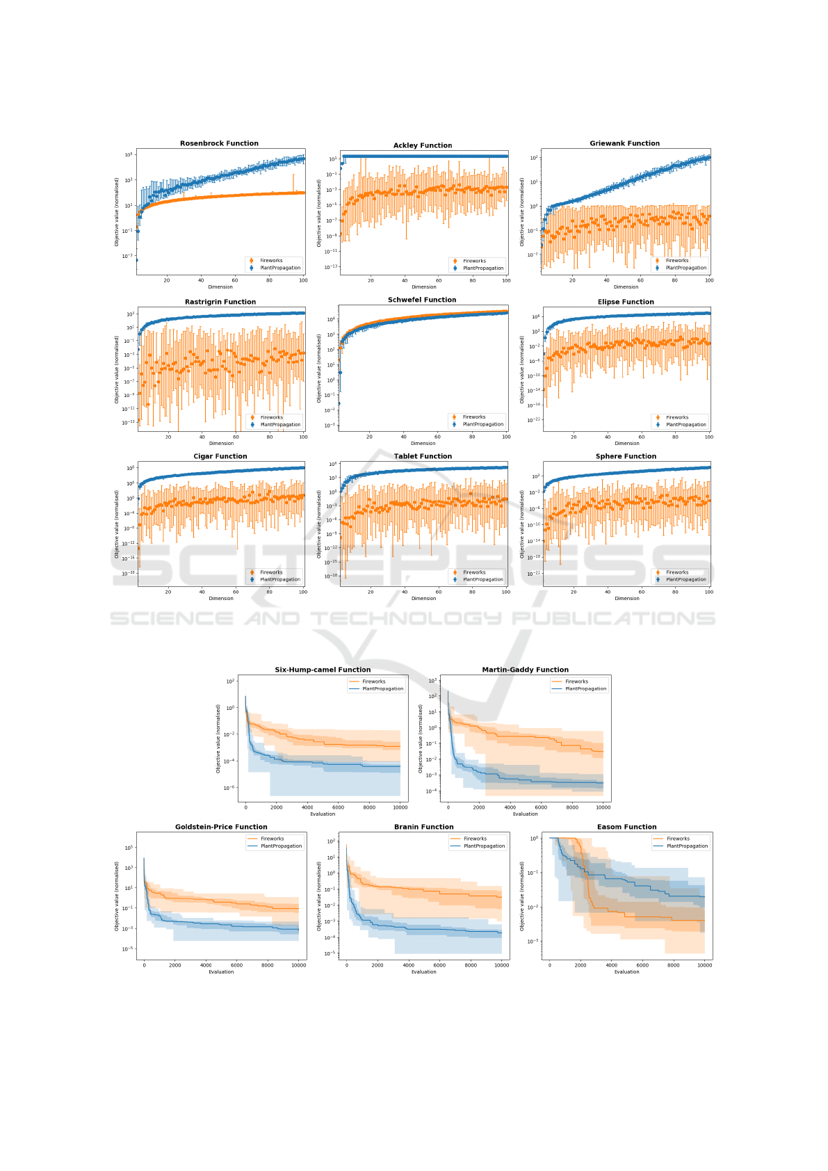
Figure 2: Normalized benchmark scores for the nine N-dimensional benchmark test functions. The horizontal axes show the
number of dimensions of the benchmark function, while the vertical axes show the median best values found after 10,000
evaluations (N = 20). The error bars show the lowest and highest achieved results (0th and 100th percentile).
Figure 3: Results for the five 2-dimensional benchmark test functions. The horizontal axes show the number of evaluations of
the benchmark function, while the vertical axes show the median best values found (N = 20). Filled areas show quartiles.
ECTA 2019 - 11th International Conference on Evolutionary Computation Theory and Applications
108

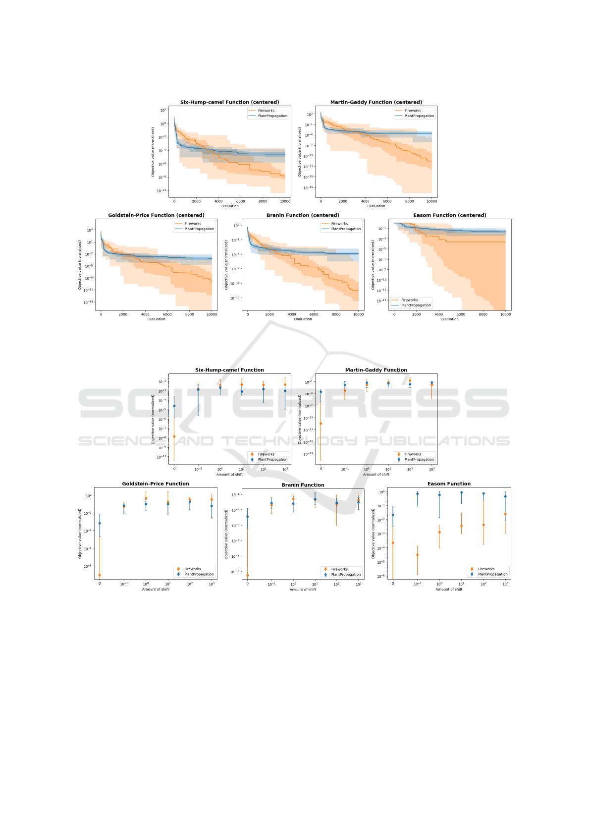
Figure 4: Results for the five centered 2-dimensional benchmark test functions. The horizontal axes show the number of
evaluations of the benchmark function, while the vertical axes show the median best values found ( N = 20 ). Lower values are
considered better. The filled areas show the quartiles.
Figure 5: Results for the five 2-dimensional benchmarks when they are translated with different values. The horizontal axes
show the amount of translation of the benchmark function, while the vertical show the median best values found ( N = 20 ).
Lower values are considered better. The error bars show the lowest and highest achieved results (0th and 100th percentile).
tive values of FWA have high variance and results can
vary as much as a factor 10
10
between trials. Results
of PPA generally have lower variance, but it seems to
be affected more by an increase in dimensionality than
FWA. PPA is unable to find good values on the Ackley
function for everything but the lowest dimensions.
Figure 3 shows normalized benchmark scores on
the five 2D functions, where PPA outperforms FWA
in four out of five cases. Both algorithms generally
converge very quickly in the first 1,000 function evalu-
ations, after which convergence speed slows down con-
siderably. In figure 4 the results for the same functions
with the minimum shifted onto the origin (‘centered’)
Fireworks Algorithm versus Plant Propagation Algorithm
109

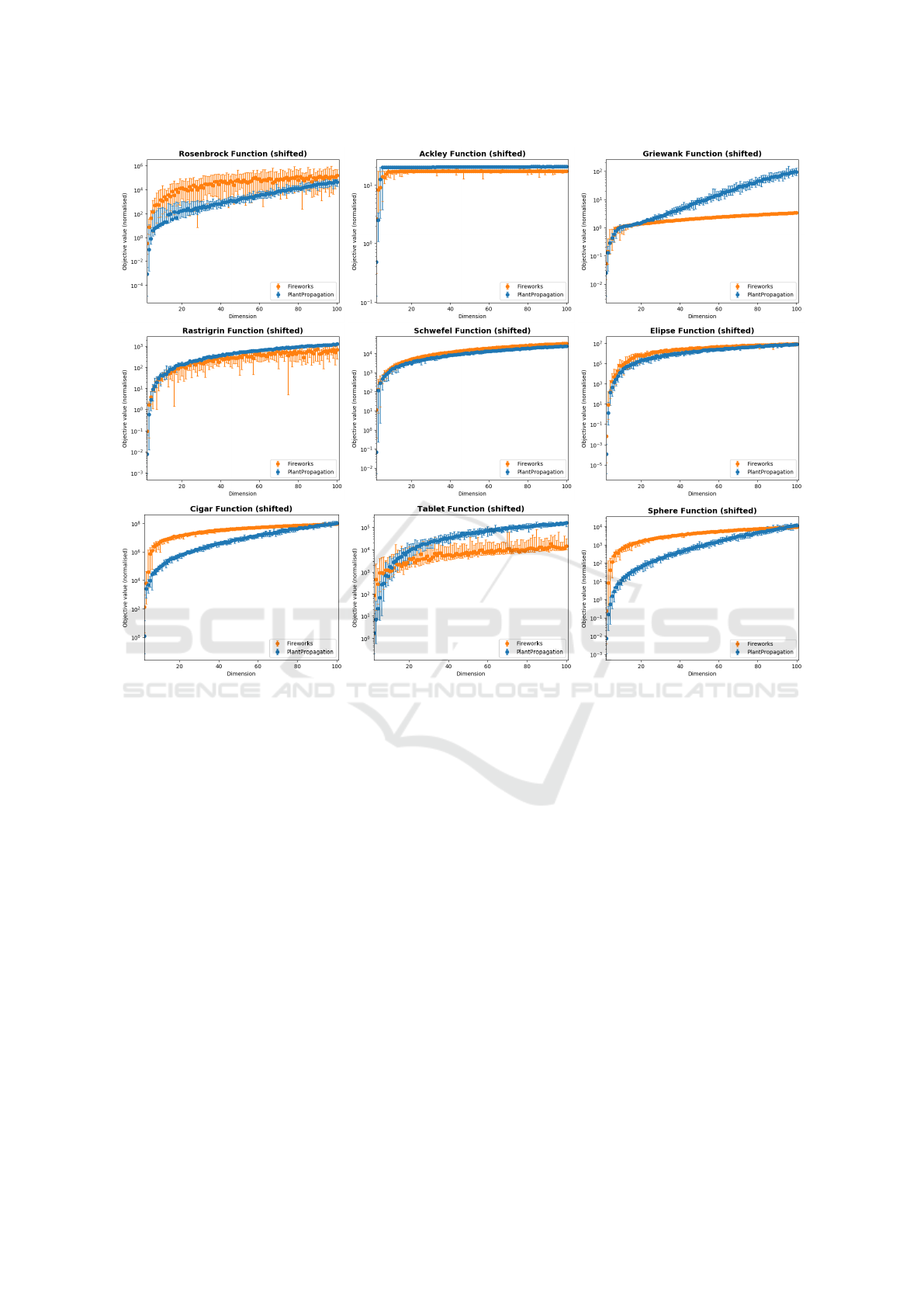
Figure 6: Normalized benchmark scores for the nine N-dimensional benchmark test functions when shifted such that the global
minimum is at x
∗
= (−10)
D
. The horizontal axes show the number of dimensions of the benchmark function, while the vertical
axes show the median best values found after 10,000 evaluations ( N = 20 ). Lower values are considered better. The error bars
show the lowest and highest achieved results (0th and 100th percentile).
are shown. In this second figure, FWA outperforms
PPA, but the high variance of FWA reappears. Statisti-
cal analysis using the Mann-Whitney U test confirms
that the newly obtained objective values are signifi-
cantly different for FWA, whereas those for PPA there
is no significant difference (FWA gives p < 0.05 , while
PPA gives p > 0.05).
To see the effect of the translation distance, a set
of six translations of different magnitudes is applied
to all centered 2-dimensional functions. Results are
shown in figure 5. As the function’s global minimum
benchmark is shifted further away from the origin, the
performance of FWA deteriorates, while PPA does not
seem to be affected. The effects of the translation ap-
pear to be the least significant on Easom, where the
performance of FWA starts deteriorating with transla-
tions greater than 1 . Note that, like shown in figures
2, 3, and 4, the variance of FWA decreases when the
global optimum is shifted away from the origin. Oth-
erwise, the variance of FWA is similar to PPA’s. The
astute observer might notice that PPA’s performance
also deteriorates slightly when the global minimum
of the benchmark function is shifted away from the
origin – which would indicate a locational bias – but
this difference cannot be proven to be significant.
For the translated N-dimensional benchmark test
functions, a translation of +10 was used over all di-
mensions (figure 6). Compared to the results in figure
2, results of both algorithms are much more similar
and FWA achieves better results than PPA on four out
of nine benchmark test functions. Most noteworthy is
the visual difference in the results of FWA between the
untranslated and the translated benchmark test func-
tions in figures 2 and 6 respectively. This difference is
not apparent in the results of PPA. This is confirmed
for all benchmark functions except Rosenbrock and
Schwefel through statistical analysis using the Mann-
Whitney U test. On Rosenbrock, Rastrigrin and Tablet,
FWA again seems to have more variability in its end
results. On the other functions however, the variance
ECTA 2019 - 11th International Conference on Evolutionary Computation Theory and Applications
110

Figure 7: Average computing time in seconds to complete
10,000 evaluations in FWA and PPA ( N = 20 ). Average
is taken only from the N-dimensional benchmarks without
applying translation. The horizontal axis shows the number
of dimensions of the benchmark test functions, and the ver-
tical axes the average time taken. The error bars show one
standard deviation.
of FWA now seems to be similar and sometimes even
smaller than that of PPA. Furthermore, FWA seems to
generally scale better than PPA when the dimensional-
ity of the problem increases.
A final notable difference is the computing times of
the algorithms (figure 7). The runtime for 10,000 eval-
uations averaged over all N-dimensional benchmark
test functions ( N = 20 ) of FWA and PPA has been
compared by fitting a straight line. Fits were tight with
a correlation coefficient of 0.927 and a standard error
of 1.371 ∗10
−3
for FWA and a correlation coefficient
of 0.980 and a standard error of 9.998 ∗10
−5
for PPA.
Thus, both algorithms increase linearly with the di-
mensionality of the benchmark test function. However,
gradients were 0.441 for FWA and 0.064 for PPA, in-
dicating that FWA slows down almost seven times as
fast when the number of dimensions is increased. The
intersects were 2.104 and 0.173 for FWA and PPA
respectively, indicating that FWA takes significantly
more time to create and evaluate an initial population.
5 DISCUSSION
Although FWA and PPA have quite similar algorithmic
paradigms, their performance is quite different. FWA
outperforms PPA as long as a function’s minimum is
at the origin, but things notably change when this is
not the case. In general, it looks like PPA is more
suitable for low-dimensional problems, but again, the
location of the global minimum seems to be of crucial
importance. An avenue of further research might in-
volve further exploring the influence of the magnitude
of these shifts. However, the magnitude of the distance
between the global minimum and the origin seems to
have little effect. Generally speaking, it seems like
FWA is more suitable for situations where dimension-
ality is high, whereas for low-dimensional problems
PPA is the better option.
Especially for FWA, multiple repetitions are ad-
vised when searching for the global optimum, as re-
sults might have high variance. It appears to converge
faster than PPA in most cases, but this is at the cost
of an increase in computational costs. Possible causes
of the high computational cost of FWA are the sub-
routines for generating Gaussian offspring, bounds
correction (using modulo), and the selection of indi-
viduals ( O(n
2
) , versus O(1) in PPA). In some real-life
problems the computational cost of evaluating the ob-
jective function is multiple orders of magnitude larger
than the computational cost of the algorithm (Keane,
1996; Ygge and Akkermans, 1996). In this case, the
most important property of a combinatorial optimiza-
tion algorithm is that it converges in as few evaluations
as possible.
Arguably, the most interesting result of this study
is the preference of FWA for centered benchmark test
functions. There seems to be a universal pattern: when
a function has its global minimum (further) away from
the origin, PPA performs better and FWA behaves less
erratic. The performance of FWA deteriorates signif-
icantly within translations within the size of 1 , and
larger translations seem to not have much more effect.
The preference of FWA for benchmark test functions
that have a global minimum positioned on the origin
was also observed by Zheng et al. (2013), but while
improvements were made in that study, the exact be-
haviour of this bias has not yet been studied. To this
end, a more general method for detecting biases in con-
tinuous optimization algorithm needs to be developed,
or as S
¨
orensen (2015) states: “Perhaps a set of tools
is needed, i.e., a collection of statistical programs or
libraries specifically designed to determine the rela-
tive quality of a set of algorithms on a set of problem
instances.”.
The source code for algorithms, benchmark test
functions, statistical methods, and graphs used in this
study is provided on GitHub (Vrielink, 2019) and may
be freely used by anyone who wishes to compare the
results of these or other optimization algorithms.
ACKNOWLEDGEMENTS
The authors would like to thank Marcus Pfundstein
(former student, UvA) for his preliminary work com-
piling a set of benchmarks, Quinten van der Post (col-
Fireworks Algorithm versus Plant Propagation Algorithm
111

league, UvA) for allowing us to use his server as a
computing platform, Hans-Paul Schwefel (Professor
Emeritus, University of Dortmund) for answering our
questions about the Schwefel benchmark function by
email, and Ying Tan (Professor, Peking University),
Abdellah Salhi (Professor, University of Essex), and
Eric Fraga (Professor, UCL London) for answering
our questions on FWA and PPA respectively.
REFERENCES
Alba, E. and Dorronsoro, B. (2005). The explo-
ration/exploitation tradeoff in dynamic cellular genetic
algorithms. IEEE transactions on evolutionary compu-
tation, 9(2):126–142.
Audibert, J.-Y., Munos, R., and Szepesv
´
ari, C. (2009).
Exploration–exploitation tradeoff using variance es-
timates in multi-armed bandits. Theoretical Computer
Science, 410(19):1876–1902.
Cheraitia, M., Haddadi, S., and Salhi, A. (2017). Hybridizing
plant propagation and local search for uncapacitated
exam scheduling problems. International Journal of
of Services and Operations Management.
El-Beltagy, M. A. and Keane, A. J. (2001). Evolutionary
optimization for computationally expensive problems
using gaussian processes. In Proc. Int. Conf. on Artifi-
cial Intelligence, volume 1, pages 708–714. Citeseer.
Geem, Z. W., Kim, J. H., and Loganathan, G. V. (2001). A
new heuristic optimization algorithm: harmony search.
simulation, 76(2):60–68.
Geleijn, R., van der Meer, M., van der Post, Q., and van den
Berg, D. (2019). The plant propagation algorithm on
timetables: First results. In Evostar 2019 “The Leading
European Event on Bio-Inspired Computation”.
Glover, F. (1989). Tabu search—part i. ORSA Journal on
computing, 1(3):190–206.
Glover, F. (1990). Tabu search—part ii. ORSA Journal on
computing, 2(1):4–32.
Imran, A. M. and Kowsalya, M. (2014). A new power system
reconfiguration scheme for power loss minimization
and voltage profile enhancement using fireworks algo-
rithm. International Journal of Electrical Power &
Energy Systems, 62:312–322.
Ishii, S., Yoshida, W., and Yoshimoto, J. (2002). Control of
exploitation–exploration meta-parameter in reinforce-
ment learning. Neural networks, 15(4-6):665–687.
Keane, A. (1996). The design of a satellite beam with en-
hanced vibration performance using genetic algorithm
techniques. Journal of the Acoustical Society of Amer-
ica, 99(4):2599–2603.
Kirkpatrick, S., Gelatt, C. D., and Vecchi, M. P. (1983).
Optimization by simulated annealing. science,
220(4598):671–680.
Li, J., Zheng, S., and Tan, Y. (2014). Adaptive fireworks
algorithm. In Evolutionary Computation (CEC), 2014
IEEE Congress on, pages 3214–3221. IEEE.
Moshrefi-Torbati, M., Keane, A., Elliott, S., Brennan, M.,
and Rogers, E. (2003). Passive vibration control of a
satellite boom structure by geometric optimization us-
ing genetic algorithm. Journal of Sound and Vibration,
267(4):879–892.
Paauw, M. and van den Berg, D. (2019). Paintings, polygons
and plant propagation. In International Conference on
Computational Intelligence in Music, Sound, Art and
Design (Part of EvoStar), pages 84–97. Springer.
Salhi, A. and Fraga, E. S. (2011). Nature-inspired opti-
misation approaches and the new plant propagation
algorithm.
Selamo
˘
glu, B.
˙
I. and Salhi, A. (2016). The plant propaga-
tion algorithm for discrete optimisation: The case of
the travelling salesman problem. In Nature-inspired
computation in engineering, pages 43–61. Springer.
S
¨
orensen, K. (2015). Metaheuristics—the metaphor exposed.
International Transactions in Operational Research,
22(1):3–18.
Storn, R. and Price, K. (1997). Differential evolution–a
simple and efficient heuristic for global optimization
over continuous spaces. Journal of global optimization,
11(4):341–359.
Sulaiman, M., Salhi, A., and Fraga, E. S. (2014a). The plant
propagation algorithm: modifications and implementa-
tion. arXiv preprint arXiv:1412.4290.
Sulaiman, M., Salhi, A., Selamoglu, B. I., and Kirikchi,
O. B. (2014b). A plant propagation algorithm for con-
strained engineering optimisation problems. Mathe-
matical Problems in Engineering, 2014.
Tan, Y. and Zhu, Y. (2010). Fireworks algorithm for opti-
mization. In International Conference in Swarm Intel-
ligence, pages 355–364. Springer.
Vrielink, W. (2019). FWA versus PPA. https://github.com/
WouterVrielink/FWAPPA.
Weyland, D. (2015). A critical analysis of the harmony
search algorithm-how not to solve sudoku. Operations
Research Perspectives, 2:97–105.
Ygge, F. and Akkermans, J. M. (1996). Power load man-
agement as a computational market. H
¨
ogskolan i Karl-
skrona/Ronneby.
Zheng, S., Janecek, A., Li, J., and Tan, Y. (2014). Dy-
namic search in fireworks algorithm. In Evolutionary
Computation (CEC), 2014 IEEE Congress on, pages
3222–3229. IEEE.
Zheng, S., Janecek, A., and Tan, Y. (2013). Enhanced fire-
works algorithm.
ECTA 2019 - 11th International Conference on Evolutionary Computation Theory and Applications
112