Deep Learning Analysis for Big Remote Sensing Image Classification
Imen Chebbi
1,2
, Nedra Mellouli
1
Myriam lamolle
1
and Imed Riadh Farah
2
1
LIASD Laboratory, University of Paris 8, Paris, France
2
RIADI Laboratory, University Of Manouba, Manouba, Tunisia
Keywords:
Big Data, Deep Learning, Remote Sensing, Classification, Spark, Tensorflow.
Abstract:
Large data remote sensing has various special characteristics, including multi-source, multi-scale, large scale,
dynamic and non-linear characteristics. Data set collections are so large and complex that it becomes difficult
to process them using available database management tools or traditional data processing applications. In
addition, traditional data processing techniques have different limitations in processing massive volumes of
data, as the analysis of large data requires sophisticated algorithms based on machine learning and deep learn-
ing techniques to process the data in real time with great accuracy and efficiency. Therefore Deep learning
methods are used in various domains such as speech recognition, image classifications, and learning methods
in language processing. However, recent researches merged different deep learning techniques with hybrid
learning-training mechanisms and processing data with high speed. In this paper we propose a hybrid ap-
proach for RS image classification combining a deep learning algorithm and an explanatory classification
algorithm. We show how deep learning techniques can benefit to Big remote sensing. Through deep learning
we seek to extract relevant features from images via a DL architecture. Then these characteristics are the entry
points for the MLlib classification algorithm to understand the correlations that may exist between character-
istics and classes. This architecture combines Spark RDD image coding to consider image’s local regions,
pre-trained Vggnet and U-net for image segmentation and spark Machine Learning like random Forest and
KNN to achieve labeling task.
1 INTRODUCTION
Earth observation is a source of information in many
fields of application such as remote sensing, cartogra-
phy, aeronautics, etc. Over the years, the number of
floating sensors in space is growing, hence the prolif-
eration of captured images. The various spaceborne
and airborne sensors deliver a large number of earth
observation data every day so that we can observe its
different sides (M.Chi, 2016). Indeed, these data are
the main actor of big remote sensing data (BRSD) and
has at least these classic 4Vs : The volume, the veloc-
ity, the veracity and the variety(I. Chebbi, 2015).
Currently, the most active research area in ma-
chine learning (ML) is deep learning (DL). With its
increased processing power and advances in proces-
sors and as the quantity of remote sensing data keeps
rising, we are starting to talk about BRSD DL. It
comes to play a major role in providing big remote
sensing data analytic solutions for classification and
clustering. Obviously, DL uses deep architectures
in order to deal with complex relationships between
the input data and the class label. In addition, DL
and ensemble-based architectures are the most pop-
ular and efficient approaches for multi-source and
multi-temporal land cover classification. They out-
perform traditional machine learning methods and
cover both optical images or radar images. DL al-
gorithms are shown better performance from hyper-
spectral and multispectral imagery such as extracting
land cover types (N.Kussul, 2017), pixel-based classi-
fication, semantic segmentation, or target recognition.
They learn features from the data, where in the bottom
level,low-level features are extracted from texture and
spectral information, and the output features are rep-
resented at the top level. In fact, DL has many well-
established deep architectures like Deep Belief Net-
work (DBN), Recurrent Neural Network(RNN), or
Convolutional Neural Network(CNN).In image pro-
cessing the most used architecture is Convolutional
Neural Networks(CNN). This architecture is multi-
layer network, composed of 2 stages: Feature extrac-
tor and classifier. Many experiments have shown that
the performance of remote sensing(RS) image scene
classification has been significantly improved due to
the powerful feature representation learnt through dif-
Chebbi, I., Mellouli, N., lamolle, M. and Farah, I.
Deep Learning Analysis for Big Remote Sensing Image Classification.
DOI: 10.5220/0008166303550362
In Proceedings of the 11th International Joint Conference on Knowledge Discovery, Knowledge Engineering and Knowledge Management (IC3K 2019), pages 355-362
ISBN: 978-989-758-382-7
Copyright
c
 2019 by SCITEPRESS – Science and Technology Publications, Lda. All rights reserved
355

ferent DL architectures (X.Chen, 2014).
The most two devoted frameworks useful in deep
learning are TensorFlow and Apache Spark. Tensor-
Flow is an open source framework which is desig-
nated to ML and especially to DL. It has built-in sup-
port for DL and Neural Network (NN), so it makes
easy to assemble a network, assign parameters and
run the training process. Also, Tensorflow has a col-
lection of samples trainable mathematic functions that
are usefull for NN. Due to the large collection of flex-
ible tools,TensorFlow is compatible with many vari-
ant of ML. In addition, TensorFlow (P.Goldsborough,
2016) uses CPUs and GPUs for computing and that’s
what make the compile time faster. Apache Spark is
also an open source parallel computing framework,
which has the advantage of MapReduce (I.Chebbi,
2018). It delivers flexibility, scalability and speed to
meet the challenges of big Data. Spark integrates two
main libraries SQL for querying large and structured
data and MLlib involving main learning algorithms
and statistical methods (A.Gupta, 2017). Obviously,
MLlib is Spark’s open-source ML library which in-
cludes several efficient functionalities for training. It
also supports different languages and provides a high-
level API that rich Spark’s ecosystem and facilitate
the development of ML pipelines (X.Meng, 2016).
The purpose of our work is to combine the perfor-
mance of two CNN models in analyzing and classify-
ing heterogeneous multi-source remote sensing data.
We decide to use four different datasets according to
image acquisition, image resolution and image encod-
ing in the perspective to evaluate the improvement of
these two architectures.
The rest of this paper is organized as follows. In
Section II, we introduce the related work. Section
III we present the proposed approach. Section IV
presents our results. A brief conclusion with recom-
mendations for future studies is presented in Section
V.
2 RELATED WORK
Deep learning is taking off in remote sensing and
many papers have been released talking about mul-
tiple applications of deep learning in remote sens-
ing. As DL a deep feature learning architecture,
it can learn semantic discriminative features and
reach better classification compared with mid-level
approaches. In (N.Kussul, 2017) a multilevel deep
learning architecture is proposed using multitemporal
images acquired by Landsat-8 and Sentinel-1A satel-
lites. The proposed architecture is a four-level ar-
chitecture, including preprocessing (level 1), super-
vised classification (level 2), post processing (level 3)
and final geospatial analysis (level 4). 1-D and 2-D
CNNs architectures are proposed to explore spectral
and spatial features. At the preprocessing level, Self-
organizing Kohenen maps (SOMs) are chosen for
optical image segmentation and restoration of miss-
ing data. SOMs are trained for each spectral band
separately. The restoration of the missing values is
done by substituting input sample missing compo-
nents with neuron’s weight coefficient. The restored
pixels are lately masked. In the second level (Super-
vised Classification with CNN), two different CNN
architectures are compared: 1-D CNN in which con-
volutions are in the spectral domain and 2-D CNN in
which convolutions is in the spatial domain. These
two architectures are composed of two convolutions
layers, max pooling layer and two fully connected
layers. The two architectures use different train fil-
ters and different number of neurons in the hidden
layers. A combination of AdaGrad and RMSProp
are used for moment estimation and it proved better
performance in term of fast convergence comparing
to gradient descent or stochastic gradient descent. In
the final level, (Postprocessing and Geospatial Anal-
ysis)several filtering algorithms have been developed
and they are based on the information quality of the
input data and field boundaries. It takes a pixel based
classification map. Finally, the data fusion allows the
interpretations of the classification methods. Another
work proposed by Nguyen et al. (T.Nguyen, 2013)
in which they considered a method for satellite im-
age classification using CNN architecture. First of all,
they converted the input image to gray and resize it
They used 3 convolutional layers and two sampling
layers. The first convolutional layer executes the con-
volution operation using five kernels 5*5 and five bi-
ases to produce five maps. The next layer is a sam-
pling layer it computes spatial subsampling for each
map of the first convolutional layer. The number of
maps of the convolutional layer is equal to the num-
ber of maps in the sampling layer. Five weights and
five biases are used in order to provide 5 maps. In the
second convolutional layer, two maps are convolved
in the second sampling layer to calculate a single map
and Therefore 10 maps are utilized in the third convo-
lutional layer. By the same way, the second sampling
layer has 10 maps. The final convolutional layer uses
10*10 kernel maps where each map was convolved
with the previous sampling layer maps and we obtain
100 maps with 1*1 sizes. This layer is fully con-
nected with the output layer which provide a vector
whose dimension is equal to the number of classes
(T.Nguyen, 2013).
In (G.Cheng, 2018) features are used directly
KDIR 2019 - 11th International Conference on Knowledge Discovery and Information Retrieval
356

from the FCN(Fully Convolutional Network) as the
classifier inputs. In contrast Duan et al. (Y.Duan,
2017) proposed an approach in which CNN pooling
layer is substituted with a wavelet constrained pool-
ing layer. This layer is used in conjunction with
Markov Random Field and superpixel in order to pro-
vide a segmentation map. In (J. Geng and Chen,
2015) Geng et al. Used deep convolutional autoen-
coders (DCAE) for extracting features and automatic
classification on high resolution single polarization
TerraSAR-X images. The architectures of the DCAE
contains a convolutional hand-crafted first layer, in
which there are kernels, and a scale transformation
hand-crafted second layer, in which the correlated
neighbor pixel is integrated. The other layers are
trained with SAE (Stacked autoencoder). In fact, Xi-
aorui Ma et al (X.Ma, 2017) proposed a classifica-
tion approach based on three decisions: the first de-
cision is a local decision. A hyperspectral image will
be sampled and the test sample is based on its neigh-
borhood by calculating the Euclidean distance. The
second decision, is a global decision based on a su-
pervised classification. It calculates an Euclidean dis-
tance between the sample and the classes. The final
decision, is a self-decision. It is based on the label
class involving spectral and spatial features. The first
two decisions are applied to unlabeled samples in the
training set. After that, the deep network is trained on
the new training set to extract features and a classifi-
cation map is generated from the self-decision. Ob-
viously, the most common challenge of RS applica-
tions is RS image classification. In fact, RS images
can have similar appearance but it belongs to differ-
ent classes. Indeed, in the few recent years the DL
approaches comes as a solution to this challenge. DL
is proving that it has efficient results in hyperspectral
and multispectral BRSD imagery in land cover types
such as extracting forests, buildings, roads.
As the DL approaches are taking off big data and re-
mote sensing. In our paper, we are going to use DL
in BRSD classification by identifying and classify-
ing objects in satellite images and executing DL algo-
rithms based on two CNN models (vggnet and U-net).
From the state of the art, the vggnet architec-
ture appears as the network devoted to feature extrac-
tion tasks. This network receives an error of about
8.5% on the ImageNet Large Scale Visual Recogni-
tion Competition (ILSVRC). This is about 1% more
than the 19-layer version, but in the interest of eas-
ier handling and computation speed. The vggnet
was chosen over Alexnet and other architectures for
its simplicity, uniform 3x3 convolutions and depth,
which gives the power to exploit more general fea-
tures. Vggnet was chosen on Resnet, with about 3.5%
on the ILSVRC once again in the interest of simplic-
ity and computational flexibility. The vggnet network
was formed (by the original authors) on Imagenet’s
well-known ILSVRC-2012 dataset (J. Deng, 2010),
consisting of 1.3 million images, distributed in 1000
classes, which makes it a good features extractor.
According to the study of art, DeepUnet and U-net
model is the most suitable for the processing of mul-
tispectral satellite images so we chose to work with
U-net for the multispectral images segmentation and
classification.
We remember that our aim in this study is to char-
acterize image objects given their labels. We con-
sider this task as object extraction from satellite image
datasets.
Furthermore, we work with four databases com-
posed of heterogeneous satellite images like RGB im-
ages, multispctral images, multi-band images with
different sizes and resolutions in order to apply two
dimensions of big data such as Volume and Variety.
3 PROPOSED APPROACH
BRSD (big remote sensing data)represents a chal-
lenge for the DL. In fact, BD involves large number
of samples as inputs, large varieties of classes as out-
puts and high large dimensionality as attributes This
will lead to high running time and model complexi-
ties. For all these reasons algorithms with distributed
framework and parallelized machines are required.
From Hubel and Wiesel’s point of view exposed in
their early work on the cat’s visual cortex (D.Hubel,
1968),we approve that the visual cortex contains a
complex arrangement of cells. These cells are sen-
sitive to small local regions of the visual field, named
a receptive field. The local regions are tiled to hedge
the whole visual field area. These cells act as local
filters and are suitable to exploit the strong spatially
local correlation present in images.
Based on this assessment, we proposed our ap-
proach in three steps as following in Figure 1. First we
propose to use Resilient Distributed Datasets (RDD)
structure of Spark wherein each image is considered
as a dataset element. Hence each image is represented
by a vector of RDDs records reflecting a local region
of the image source. When the RDDs vectors are es-
tablished, they are forwarded to the deep neural net-
work inputs wherein the number of networks is equal
to each vector dimension. At this second step, we
are looking for local-object identification and image
segmentation by using a pre-trained Vggnet network.
At the third step we pipeline the Vggnet outputs to a
random forest and KNN machine learning with ML-
Deep Learning Analysis for Big Remote Sensing Image Classification
357

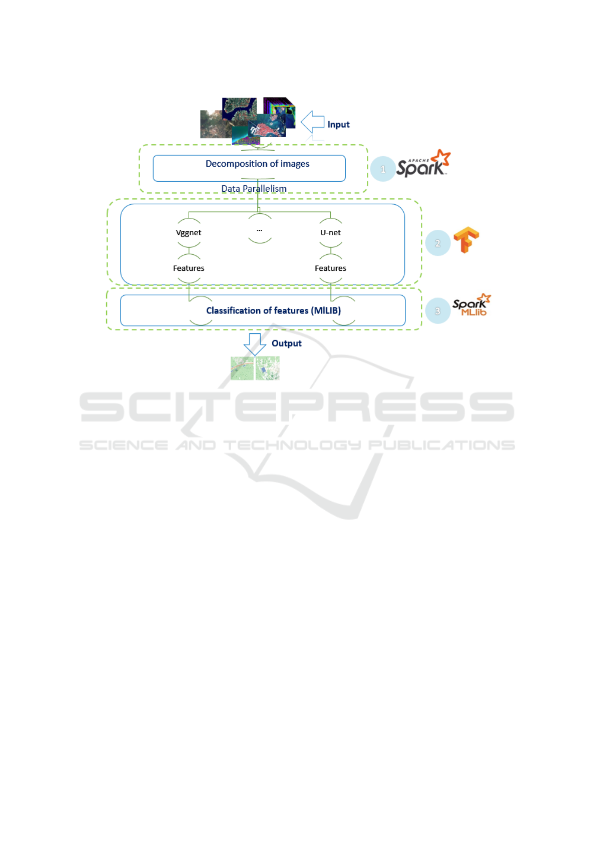
Figure 1: The Proposed Approach.
lib package to aggregate and to reach the final image
class.
3.1 Loading Images into Spark Data
Frame (c.f Figure1)
The 1st step consists in loading millions of RS im-
ages into Spark Resilient Distributed Dataset (RDD).
Then, the data is decoded in a distributed Platform
dedicated to large scale manipulation using Tensor-
Flow as DL library on each distributed worker in or-
der to test the hyper-parameters RDD of the model
and also to speed up the time intensive task with
Spark.
Spark addresses data distribution by integrating
the RDDs concept. Therefore each partition remains
in memory on its server .i.e. RS data is incorporated
in stripes into the RDDs. HDFS key/value are gen-
erated to each image partition to overcome the data
heterogeneity thus HDFS yields BRSD storage with
high read throughput.
3.2 Feature Extraction and Image
Segmentation (c.f Figure1)
The second step involves two stages: Object identifi-
cation and image segmentation. At this stage, we used
DL.
After studying multiple works, we choose to work
with vggnet as the most efficient model for RGB re-
mote sensing data and U-net as the most efficient
model for multispectral data.
3.2.1 Object Identification
For the object identification we used pre-trained
vggnet-16. In order to get a model which is adapted
for our need we fine-tuned the model. Fine-tuning is
one of the most important methods for creating a large
scale model. Indeed, this technique uses an already
formed network and allows to redefine any compo-
nents(weights, layers,outputs) according to the new
data set.
For our approach, we have used a pre-trained
vggnet-16. The network is composed of 22 lay-
ers, 16 layers with learnable weights (13 convolu-
tional layers, and 3 fully connected layers). We have
adapted the configuration of the input to consider any
RGB satellite image with any resolution (instead of
224x224).
In order to get a model adapted to our need we
fine-tuned the model. Fine-tuning is one of the most
important technique devoted to a large scale model.
Indeed, this technique uses a pre-trained network and
KDIR 2019 - 11th International Conference on Knowledge Discovery and Information Retrieval
358

allows to scale any component (weights, layers, out-
puts) according to the new data set. Finally, to have
an output adapted to our problem we have re-trained
only 3 output dense layers. Since we use vggnet-16 as
a feature extractor, the layers we are going to freeze
are the first 22 layers.
After performing the model fine-tuning phase, we
retrieve the characteristics from the last ”block5pool”
layer. We then use these characteristics and send
them to dense layers formed according to our dataset.
When the output layer of the pre-trained vggnet-16 is
a SOFTMAX activation with 1000 classes, we have
adapted this layer to 10 classes of SOFTMAX layer
(Buildings, cars, crops, Fast H2O, roads, Slow H2O,
Structures, Tracks, Trees and Trucks). Therefore we
have simply trained the weights of these layers and
have tried to identify the objects.
A U-net architecture is like a convolutional au-
toencoder, but it also has skip-like connections with
the feature maps located before the bottleneck (com-
pressed embedding) layer, in such a way that in the
decoder part some information comes from previous
layers, by passing the compressive bottleneck. The
output represents a segmentation map that can be used
for the segmentation part(next step).
U-Net architecture is based on encoders and de-
coders. The encoder gradually reduces the spatial
dimension with pooling layers and decoder gradu-
ally recovers the object details and spatial dimension.
There are usually shortcut connections from encoder
to decoder to help it to recover the object details bet-
ter.
3.2.2 Image Segmentation
Image segmentation is a subject of automatic learning
in which we have not only to classify what we have
seen in an image, but also to do it at the pixel level.
The aim of the classification task is to reach carto-
graphic representation from a satellite image wherein
the elements are automatically grouped by their val-
ues.
This step of the process is applied to multispec-
tral images. Over the years, many techniques have
allowed the segmentation of images using convolu-
tional neural networks (CNN).
A general semantic segmentation architecture can
be broadly thought of as an encoder network fol-
lowed by a decoder network: The encoder is usually
a pre-trained classification network like pre-trained
Vggnet-16 followed by a decoder network, and the
task of the decoder is to semantically project the dis-
criminative features (lower resolution) learnt by the
encoder into the pixel space (higher resolution) to get
a dense classification.
U-net is an encoder-decoder architecture, we have
used it for the segmentation step. This U-net pre-
trained architecture is adapted to handle with multi-
spectral images.
A U-net with batch normalization is developed in
Tensorflow and serves as a segmentation model. The
model was formed for 9,000 lots, each batch contain-
ing 60 image patches. Each image area corresponds
to a crop of 144*144 from the original images.
Similar to the original U-net architecture, the loss
is calculated only on the 80 * 80 center region, be-
cause the edge pixels receive only partial information.
The model has been applied to satellite images
with 20 bands rather than 3 bands, a part from the
information provided by the RGB bands the other 20
bands contain much more information about the neu-
ral network to reflect, thus facilitating learning and the
quality of predictions: he is aware of the visual char-
acteristics that man does not possess. The additional
bands of available light are called P, M and A bands.
3.3 Image Classification (c.f Figure1)
After identifying objects of the given images, we must
now perform the classification step. To do it, we used
two different algorithms from Spark’s machine learn-
ing library(MLlib), namely Random Forest and KNN
(K-Nearest Neighbor).
the outputs of vggnet and U-net are pipelined to
the input of this step.
4 EXPERIMENTAL RESULTS
In this section, we will present some experimental se-
tups and results.
4.1 Experimental Setup
4.1.1 Hardware and Software Description
Our algorithm is preforming on 2 machines with
Ubunto 16.07 operating system installed NVIDIA
GEFORCE GTX 950M graphic device 8GByte
graphic memory and AWS server machine p2.xlarge
provide up to 16 NVIDIA K80 GPUs, 64 vCPUs
and 732 GiB of host memory, with a combined 192
GB of GPU memory, 40 thousand parallel processing
cores, 70 teraflops of single precision floating point
performance, and over 23 teraflops of double preci-
sion floating point performance.
The algorithm is implemented using Python2.7,
Tensorflow 1.3 and Apache Spark2.3.0 with Hadoop
2.7.
Deep Learning Analysis for Big Remote Sensing Image Classification
359

4.1.2 Data Description
We have used 4 datasets to improve our approach:
SIRI-WHU , AID , multispectral dataset, and we pre-
pared a dataset which is a composed of satellite im-
ages captured with different sensors like SPOT4 ,
SPOT5, LANDSAT8 and so on.
We reorganized the SIRI-WHU and AID datasets
in order to obtain coherent datasets with 10 classes
(Buildings, cars, crops, Fast H2O, roads, Slow H2O,
Structures, Tracks, Trees and Trucks).
• SIRI-WHU Data Set. This is a 12-class Google
image dataset of SIRI-WHU meant for research
purposes. There are 200 images, each image mea-
sures 200*200 pixels, with a 2-m spatial resolu-
tion (Siri-Whu, ).
• AID Dataset. AID is a new large-scale aerial
image dataset, by collecting sample images from
Google Earth imagery. The new dataset is made
up of the following 30 aerial scene types. All im-
ages are labeled by the specialists in the field of
remote sensing image interpretation. In all, the
AID dataset has a number of 10000 images within
30 classes (Inria, ).
• Our Dataset: our dataset has a number of 3,974
images within 10 classes. The images have var-
ious resolution 600*600, 989*989, 753*753 and
1024*1024.
• Multispectral: this dataset contains 1km x 1km
satellite images in both 3-band and 16-band for-
mats. The 3-band images are the traditional RGB
natural color images. The 16-band images contain
spectral information by capturing wider wave-
length channels. This multi-band imagery is taken
from the multispectral (400-1040nm) and short-
wave infrared (SWIR) (1195-2365nm) range.
4.1.3 Evaluation Metrics
The metrics that we used in order to evaluate the
performance of our work are precision, recall, and
F1-score.
Precision =
T P
T P+FP
Recall =
T P
T P+FN
F1 − score = 2 ∗
Accuracy×Recall
Accuracy+Recall
Where TP (True Positives) denotes the number of
correctly detected objects, FN (False Negatives) the
number of non-detected objects and FP (False posi-
tives) the number of incorrectly detected objects.
4.2 Results
Our datasets are splitted into two parts 70% for the
training and 30 % for the test.
4.2.1 VGGnet
The overall results of our 3 datasets is mentioned in
the table 1below:
4.2.2 U-net
The second type of workers are destinated for the
multispectral images. The training phase the accuracy
was 0.93% The Test phase the results are mentioned
in the table 2 below:
4.2.3 Discussion
In this work, a DL implementation for identifying and
classifying objects in satellite images is presented.
The implementation has been based on two frame-
works SPARK for storing, distributing and paral-
lelizing Big Remote Data and Tensorflow for imple-
menting and executing DL algorithms based on two
CNN models (VGGnet and U-net).We used four im-
age databases from different sources to apply the 2
DL algorithms to them based on the type, number and
resolution of the bands. We have applied Vggnet on
the first three bases and encouraging results have been
obtained in particular with the Siri and our proprietary
dataset. Indeed, the images of these two databases are
in RGB or in 3 bands. While the AID dataset has a
better resolution than the other two datasets and has
exactly the same classes, it was very difficult to char-
acterize in terms of object identification. At the same
time, U-net has been applied to the the fourth dataset
and is more efficient in identifying objects from high
resolution image dataset, as is the case with the mul-
tispectral dataset.
These results suggest that some DL algorithms are
sensitive to image resolution and others to image size.
The joint use of two models within our system makes
sense given the heterogeneity of the input source im-
ages.
5 CONCLUSIONS
Big data and DL are both considered as a big deal for
researchers. The concept of DL is to burrow into a
massive volume in order to identify patterns and ex-
tract features from complex unsupervised data with-
out human intervention, which make it an important
KDIR 2019 - 11th International Conference on Knowledge Discovery and Information Retrieval
360

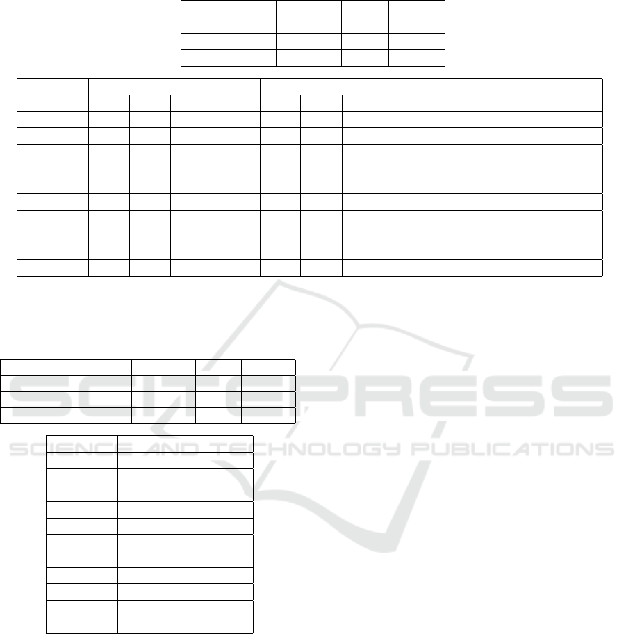
Table 1: Results obtained on 3 data sets with VGGNet model, the first table represents the results of the whole dataset and the
second table represents the results for each class.
Datasets accuracy recall FScore
SIRI 0.73 0.68 0.7
AID 0.61 0.50 0.55
Our DataBase 0.84 0.81 0.82
labels accuracy recall FScore
Siri AID Our database Siri AID Our database Siri AID Our database
Buildings 0.24 0.56 0.33 0.52 0.79 0.63 0.90 0.69 0.78
Cars 0.5 0.77 0.61 0.53 0.53 0.53 0.53 0.73 0.62
Crops 0.8 0.5 0.62 0.81 0.87 0.84 0.89 0.94 0.91
FastH2O 0.89 0.4 0.55 0.77 0.50 0.61 0.89 0.67 0.76
Roads 0.69 0.73 0.71 0.83 0.77 0.80 1 0.78 0.93
SlowH2O 0.47 0.56 0.51 0.86 0.80 0.83 1 0.79 0.88
Structure 0.6 0.3 0.57 0.75 0.75 0.75 0.64 0.88 0.78
Tracks 0.37 0.5 0.42 0.62 0.67 0.64 0.76 0.57 0.67
Trees 0.16 0.06 0.12 0.80 0.50 0.62 0.80 0.57 0.67
Trucks 0.69 0.71 0.73 0.58 0.85 0.69 0.88 0.79 0.83
Table 2: Results obtained with Unet on the multispectral
dataset results, the first table represents the results of the
whole dataset and the second table represents the results for
each class.
Datasets accuracy recall FScore
Multispectral Dataset 0.92 0.57 0.70
AID 0.71 0.68 0.69
SIRI 0.8 0.79 0.79
labels accuracy
Multispectral Dataset
Buildings 0.86
Cars 0.61
Crops 0.81
FastH2O 0.38
Roads 0.16
SlowH2O 0.46
Structure 0.94
Tracks 0.96
Trees 0.98
Trucks 0.93
tool for Big Data. This paper presents an technolog-
ical architecture for better classify sensing images.
This work contains a study of some machine learn-
ing tools to perform image classification. Specifi-
cally: the Spark Machine Learning implementations
with two pre-trained CNN (transfer learning from Vg-
gnet and U-net) were taken into account to categorize
samples from 4 datasets.A benchmark dataset of re-
mote sensing images was created for evaluation. For
the future work, we are going to use other multispec-
tral and hyperspectral Dataset for U-net results val-
idation and we are going to develop other DL archi-
tectures in order to adopt our approach to different RS
data types.
REFERENCES
A.Gupta, H.Thakur, R. P. S. (2017). A big data analysis
framework using apache spark and deep learning. In
ICDM Workshops: 9-16.
D.Hubel, T. (1968). Receptive fields and functional archi-
tecture of monkey striate cortex. In Journal of Physi-
ology (London), 195, 215243.
G.Cheng, C.Yang, X. L. J. (2018). When deep learning
meets metric learning : remote sensing image scene
classification via learning discriminative cnns. In
IEEE transactions on geoscience and remote sensing,
56(5) :28112821.
I. Chebbi, W. Boulila, I. F. (2015). Big data: Concepts,
challenges and applications. In ICCCI (2) 2015: 638-
647. SPRINGER.
I.Chebbi, W.Boulila, N. M. I. (2018). A comparison of big
remote sensing data processing with hadoop mapre-
duce and spark. In ATSIP : 1-4.
Inria, D.
J. Deng, R. Socher, L. F.-F. W. D. K. L. L. L. (2010). Spec-
tralspatial classification of hyperspectral image based
on deep auto-encoder. In IEEE Conference on Com-
puter Vision and Pattern Recognition(CVPR).
J. Geng, J. Fan, H. W.-X. M. B. L. and Chen, F. (2015).
High-resolution sar imageclassification via deep con-
volutional autoencoder. In IEEE Geoscience and Re-
mote Sensing Letters, vol. 12: 23512355.
M.Chi, A.Plaza, J. Z. J. Y. (2016). Big data for remote sens-
ing: Challenges and opportunities. In Pro-ceedings of
the IEEE 104(11): 2207-2219. IEEE.
Deep Learning Analysis for Big Remote Sensing Image Classification
361

N.Kussul, M.Lavreniuk, S. A. (2017). Deep learning clas-
sification of land cover and crop types using remote
sensing data. In IEEE Geosci. Remote Sensing Lett.
14(5): 778-782. IEEE.
P.Goldsborough (2016). A Tour of TensorFlow. CoRR
abs/1610.01178.
Siri-Whu, D.
T.Nguyen, J.Han, D. (2013). Satellite image classification
using convolutional learning. In AIP Conference Pro-
ceedings,(1558):22372240.
X.Chen, X. (2014). Big data deep learning: Challenges and
perspectives. In EEE Access 2: 514-525. IEEE.
X.Ma, H.Wang, J. (2017). Spectral-spatial classification of
hyperspectral image based on deep auto-encoder. In
IEEE Journal of Selected Topics in Applied Earth Ob-
servations and Remote Sensing.
X.Meng, J.K. Bradley, B. E. S.-S. (2016). Mllib: Ma-
chine learning in apache spark. In Journal of Machine
Learning Research 17: 34:1-34:7.
Y.Duan, F.Liu, L. P. L. (2017). Sar image segmentation
based on convolutional-wavelet neural network and
markov random field. In Pattern Recognition, 64
:255267.
KDIR 2019 - 11th International Conference on Knowledge Discovery and Information Retrieval
362