Calibration Techniques for Binary Classiﬁcation Problems: A

Comparative Analysis

Alessio Martino

, Enrico De Santis

, Luca Baldini

and Antonello Rizzi

Department of Information Engineering, Electronics and Telecommunications, University of Rome ”La Sapienza”,

Via Eudossiana 18, 00184 Rome, Italy

Keywords:

Calibration, Classiﬁcation, Supervised Learning, Support Vector Machine, Probability Estimates.

Abstract:

Calibrating a classiﬁcation system consists in transforming the output scores, which somehow state the con-

ﬁdence of the classiﬁer regarding the predicted output, into proper probability estimates. Having a well-

calibrated classiﬁer has a non-negligible impact on many real-world applications, for example decision mak-

ing systems synthesis for anomaly detection/fault prediction. In such industrial scenarios, risk assessment is

certainly related to costs which must be covered. In this paper we review three state-of-the-art calibration

techniques (Platt’s Scaling, Isotonic Regression and SplineCalib) and we propose three lightweight proce-

dures based on a plain ﬁtting of the reliability diagram. Computational results show that the three proposed

techniques have comparable performances with respect to the three state-of-the-art approaches.

1 INTRODUCTION

Classiﬁcation is one of the most important problems

falling under the machine learning and, speciﬁcally,

under the supervised learning umbrella. Generally

speaking, it is possible to sketch three main families:

clustering, regression/function approximation, classi-

ﬁcation. These problems mainly differ on the nature

of the process to be modelled by the learning system

(Martino et al., 2018a).

More into details, let P : X → Y be an orientated

process from the input space X (domain) towards the

output space Y (codomain) and let hx,yi be a generic

input-output pair drawn from P, that is y = P(x).

In supervised learning a ﬁnite set S = hX,Y i of

input-output pairs is supposed to be known and com-

mon supervised learning tasks can be divided in clas-

siﬁcation and function approximation. In the former

case, the output space Y is a non-normed space and

output values usually belong to a ﬁnite categorical set

of possible values. Conversely, in the latter case, the

output space is a normed space (usually R). In unsu-

pervised learning there are no output values and reg-

ularities have to be discovered using only informa-

https://orcid.org/0000-0003-1730-5436

https://orcid.org/0000-0003-4915-0723

https://orcid.org/0000-0003-4391-2598

https://orcid.org/0000-0001-8244-0015

tion from X . The seminal example is data clustering,

where aim of the learning system is to return groups

(clusters) of data in such a way that patterns belong-

ing to the same cluster are more similar with respect to

patterns belonging to other clusters (Jain et al., 1999;

Martino et al., 2017b; Martino et al., 2018b; Martino

et al., 2019; Di Noia et al., 2019).

Synthesizing a classiﬁer (predictive model) con-

sists in feeding some hx,yi pairs to a training algo-

rithm in such a way to automatically learn the under-

lying model structure. In other words, the classiﬁer

learns a decision function f that, given an input x, re-

turns a predicted class label ˆy, i.e. a prediction regard-

ing the class that pattern may belong to:

ˆy = f (x) (1)

Eq. (1) is usually referred to as hard classiﬁca-

tion. Probabilistic classiﬁers can also return a pos-

terior probability P(output|input) which can be use-

ful for many real-world applications, for example

condition-based maintenance, decision support sys-

tems or anomaly/fault detection as operators usually

want to know the probability of a speciﬁc equipment

to fail given some input (known) state/conditions

(De Santis et al., 2018b). Trivially, probabilistic clas-

siﬁers can be ’forced’ to return hard predictions by

letting

ˆy = argmax

P(Y = y|X) (2)

Martino, A., De Santis, E., Baldini, L. and Rizzi, A.

Calibration Techniques for Binary Classiﬁcation Problems: A Comparative Analysis.

DOI: 10.5220/0008165504870495

In Proceedings of the 11th International Joint Conference on Computational Intelligence (IJCCI 2019), pages 487-495

ISBN: 978-989-758-384-1

487

that is, for a given input pattern x ∈ X, the classiﬁer

assigns the output label y ∈ Y which corresponds to

the maximum posterior probability.

Albeit not all classiﬁers are probabilistic classi-

ﬁers, some classiﬁers such as Support Vector Machine

(SVM) (Boser et al., 1992; Cortes and Vapnik, 1995;

Sch

olkopf and Smola, 2002; Cristianini and Shawe-

Taylor, 2000) or Na

ıve Bayes may return a score s(x)

which somewhat states the ’conﬁdence’ in the predic-

tion of a given pattern x. As regards Na

ıve Bayes, this

score can be seen as the probability estimate for class

membership. However, this score is not calibrated

(Domingos and Pazzani, 1996). For SVMs, the score

is basically the distance with respect to the separat-

ing hyperplane: the sign of s(x) determines whether

x has been classiﬁed as positive or negative, whereas

the magnitude of s(x) determines the distance with re-

spect to the hyperplane. Conversely to Na

ıve Bayes,

SVMs’ scores not only are not calibrated, but also are

not bounded in [0, 1], albeit some re-scaling can be

performed (Zadrozny and Elkan, 2002).

Formally speaking, a classiﬁer is said to be well-

calibrated if P(y|s(x) = s), that is, the probability for

a pattern x to belong to a label y converges to the

score s(x) = s as the number of samples tends to inﬁn-

ity (Murphy and Winkler, 1977; Zadrozny and Elkan,

2002). In plain terms, the calibration of a classiﬁca-

tion system consists in mapping the scores (or not-

calibrated probability estimates) into proper probabil-

ity estimates bounded in range [0,1] by deﬁnition.

The aim of this paper is to investigate amongst

several calibration techniques by considering binary

classiﬁcation problems using SVM as classiﬁcation

system. The remainder of this paper is structured as

follows: in Section 2 we give an overview of exist-

ing calibration techniques and ﬁgures of merit for ad-

dressing the goodness of the calibration along with

three new lightweight procedures to be compared

with state-of-the-art approaches; in Section 3 we de-

scribe the datasets used for experiments, along with

comparative results amongst the considered methods;

Section 4 concludes the paper, suggesting future re-

search and applications.

2 AN OVERVIEW OF

CALIBRATION TECHNIQUES

2.1 Current Approaches

In order to quantify the calibration of a given classiﬁer

the reliability diagram is usually employed (Murphy

and Winkler, 1977). The reliability diagram is built as

follows:

• scores/probabilities go on the x-axis

• empirical probabilities P(y|s(x) = s), namely the

ratio between the number of patterns in class y

with score s and the total number of patterns with

score s, go on the y-axis

and if the classiﬁer is well-calibrated, then all points

lie on the y = x line (i.e., the scores are equal to the

empirical probabilities). In case of binary classiﬁ-

cation, the empirical probabilities regard the positive

instances only (i.e., the ratio between the number of

positive instances having score s and the total number

of instances with score s).

Since scores are normally real-valued scalars, it is

quite impossible to quantify the number of data points

sharing the same score

. In this case, a binning pro-

cedure is needed:

• on the x-axis, the average score value within the

bin is considered

• on the y-axis, we get the ratio between the number

of patterns in class y lying in a given bin and the

total number of patterns lying in the same bin.

In works such as (Zadrozny and Elkan, 2002) and

(Niculescu-Mizil and Caruana, 2005) the authors pro-

posed to consider 10 equally-spaced bins in range

[0,1], regardless of the distribution of the scores

within that range. For some datasets, however, this

might not be a good choice and suitable alternatives

which somewhat consider the available samples are:

• The Scott’s rule (Scott, 1979) evaluates the bin

width according to the number of samples (scores)

n and their standard deviation σ as

bin witdh =

3.5 ·σ

1/3

• The Freedman–Diaconis rule (Freedman and Dia-

conis, 1981) evaluates the bin width as follows

bin witdh =

2 ·IQR

1/3

where IQR is the inter-quantile range

• The Sturges’ formula (Sturges, 1926) evaluates

the number of bins as follows

number of bins = 1 + dlog

where d·e denotes the ceiling function

• The square root choice, where the number of bins

is given by

number of bins =



√



This counting procedure will return the (trivial) value

of 1 for any s(x).

NCTA 2019 - 11th International Conference on Neural Computation Theory and Applications

488

However, using a single binning, even if evaluated ac-

cording to one of the four alternatives above, might

not be a good choice, especially if data do not fol-

low a speciﬁc underlying distribution (e.g., uniform

distribution in case of uniform binning or normal dis-

tribution in case of the Sturges’s formula). To this

end, in (Naeini et al., 2015), the Authors proposed

the Bayesian Binning into Quantiles technique, which

considers different binning (and their combination) in

order to make the calibration procedure more robust.

Let c denote the positive class and let us assume

P(c|x) = 1 for positive patterns and P(c|x) = 0 other-

wise. After training a classiﬁer such as SVM, aim of

the calibration procedure is to ﬁnd a function f for-

mally deﬁned as

f : s(x) →

P(c|x) (3)

hence, in other words, a function (model) in charge of

transforming score values into probability estimates.

One of the most famous techniques is the Platt’s

scaling (Platt, 2000; Niculescu-Mizil and Caruana,

2005), a parametric approach in order to estimate

P(y = 1|s(x)), namely the probability that a given pat-

tern x belongs to the positive class. Platt’s discussion

starts by using the Bayes’ formula

P(y = 1|s(x)) =

p(s(x)|y = 1)P(y = 1)

∑

i={±1}

p(s(x)|y = i)P(y = i)

(4)

where P(y = i) are prior probabilities and p(s(x)|y =

i) are the class conditional densities (i.e., the prob-

ability density function for belonging to class i). In

order to use Eq. (4), one can estimate the class con-

ditional densities by considering the normalized his-

tograms of the scores as returned by the SVM. Platt

showed that if the margin between the histograms of

the two classes have an exponential trend, then Bayes’

rule leads to

P(y = 1|s(x)) =

1 + exp{As(x) + B}

(5)

which is a plain parametric sigmoid function and tun-

ing the calibration model basically consists in ﬁnd-

ing the two parameters A and B. Platt suggests to

minimize the negative log-likelihood on some train-

ing data by means of a model-trust optimization pro-

cedure based on the Levenberg-Marquardt algorithm.

In (Lin et al., 2007) an improved optimization proce-

dure based on Newton’s method is proposed. Platt’s

scaling has been proved to be successful if the relia-

bility diagram of the dataset shows a sigmoidal trend.

An alternative technique relies on isotonic regres-

sion (Zadrozny and Elkan, 2002; Zadrozny and Elkan,

2001). Pair-Adjacent Violators (Ayer et al., 1955) is

one of the main algorithms in order to compute an iso-

tonic regression. Given a real-valued vector x ∈ R

and a weights vector

w ∈ R

such that x

≥ x

i−1

and

> 0 for all i = 1,.. .,n, then the isotonic regression

of a function f (x) consists in ﬁnding a function g(x)

according to a mean squared error criterion

∑

i=1

(g(x

) − f (x

))

(6)

where g(x) must be a piecewise non-decreasing (iso-

tonic) function. By letting y and s be the vectors

containing the output class labels and their respective

scores, Pair-Adjacent Violators works as follows:

1. sort y according to s: if y is already isotonic

, then

return the estimate

y ≡ y, otherwise initialize the

estimate values as

y = y

2. if

y is not isotonic, there must exist an index i such

that

≤

i−1

: for these values

we estimate

i−1

3. repeat step 2 until

y is isotonic.

At the end of this procedure,

y contains ordered values

(probability estimates) for scores in s. Further, due

to the piecewise nature of isotonic regression,

y will

contain few different values, each of which is repeated

several times. Generally, Pair-Adjacent Violators re-

turns more samples in the score space where patterns

have been misclassiﬁed and less samples where pat-

terns have been correctly classiﬁed.

A recently proposed method is called SplineCalib

(Lucena, 2018) which aims at overcoming the major

drawbacks of Platt’s scaling and isotonic regression:

• the Platt’s scaling is based on the empirical ob-

servation that the relationship between scores and

probabilities are often well-ﬁtted by a sigmoid

function: obviously, this works well only when

the data ﬁt the model, but performs poorly when

the calibration function is not well-approximated

by a sigmoid function

• the Platt’s scaling works well for few calibration

data (less than 1000 instances), but the isotonic

regression overcomes this limitation

• the nature of piecewise constant approximation

given by isotonic regression opens to a wider fam-

ily of calibration function; however, its coarseness

can be a drawback.

This most general form is usually referred to as

weighted isotonic regression. However, in this work, the

weights vector is omitted.

All 0’s followed by all 1’s since we are considering bi-

nary classiﬁcation.

The properly-said ”pair-adjacent violators” since they

violate the isotonic trend.

Calibration Techniques for Binary Classiﬁcation Problems: A Comparative Analysis

489

As its name suggests, SplineCalib is based on (cu-

bic) smoothing splines. Like isotonic regression,

SplineCalib is a non-parametric approach and, at the

same time, unlike isotonic regression, SplineCalib ﬁts

a cubic spline instead of a piecewise constant approx-

imation. In standard spline interpolation, one chooses

a set of knots and ﬁts a polynomial (usually with de-

gree 3 or 4) within each interval: the more knots, the

better the ﬁtting of the data but also high risk of over-

ﬁtting. Smoothing splines (Wahba, 1990) may also

use all of the available points as knots and perform

a regularized penalty on the second derivative of the

function. Given a relationship between predictors x

and output y of the form y = f (x), the smoothing

spline estimate

f of f is the function, amongst the

twice-differentiable ones, that minimize

∑

i=1



−

f (x

)



+ λ

(t)dt (7)

In (Lucena, 2018), instead of minimizing the sum

of squares, the Author proposes to employ a log-

likelihood criterion instead

−

∑

i=1



·log

f (x

)) + (1 −y

) ·log(1 −

f (x

))



(t)dt (8)

which resembles logistic regression (Hastie et al.,

2001). Both Eqs. (7) and (8) see the regularization

term λ ≥ 0 which weights the contribution between

goodness of ﬁt (leftmost term) and roughness (right-

most term). Speciﬁcally, if λ →0 no smoothing is tol-

erated, with risk of overﬁtting; conversely, if λ → ∞

no curvature is tolerated, with risk of going towards

an ordinary least squares interpolation.

The probability estimates via SplineCalib can be eval-

uated by the following steps:

1. sample K knots

from the unique items in the

score vector s

2. build the natural basis expansion matrix X ∈R

n×K

between values in s and the K knots. Given a set

of ordered knots {φ

,.. .,φ

}, the natural cubic

spline basis is deﬁned as

(x) = 1

(x) = x (9)

k+2

(x) = d

(x) −d

K−1

(x) ∀k = 1,... ,K −2

where d

(x−φ

)

−(x−φ

)

−φ

3. perform an `

-regularized logistic regression over

the pair hX,yi by considering a candidate value

One can also use all the available points, yet the Author

states that 200 points sufﬁce.

set for λ and choose the best value, say λ

, as the

one that returns the best cross-validation log-loss

4. re-ﬁt hX,yi using λ

5. return the calibration function f (s) by composing

the basis expansion of s and the ﬁtted model from

the previous step in order to return the probability

estimate.

2.2 Proposed Techniques

All of the three methods explained so far share the

common goal to properly ﬁt the reliability diagram:

the better the ﬁt, the more reliable the resulting prob-

ability estimates. Whilst the three methods use the

’score–label’ pairs in order to accomplish this task, we

investigate an alternative exercise by ﬁtting the points

lying on the reliability diagram. Hence, instead of

working with ’score–label’ pairs, we work with ’aver-

age bin value–fraction of positive patterns in that bin’

pairs. As will be clear in Section 3, a reliability dia-

gram almost never shows a linear trend, hence this ﬁt-

ting shall rely on more sophisticated functions

. For

these exercises we use:

1. polynomial ﬁtting: the points lying on the relia-

bility diagram are ﬁtted by means of 3-degree and

4-degree polynomials

2. spline ﬁtting: after choosing a suitable number of

knots and considering the corresponding intervals,

within each interval a natural cubic spline interpo-

lation is performed.

2.3 Figures of Merit

It is important to quantify the goodness of the calibra-

tion, hence how the probability estimates are far from

the empirical probabilities. To this end, two meth-

ods have been proposed in literature: the Brier score

(Brier, 1950; DeGroot and Fienberg, 1983) and the

Log-Loss score.

Given a series of N known events and the respec-

tive probability estimates, the Brier score is the mean

squared error between the outcome o (1 if the event

has been veriﬁed and 0 otherwise) and the probability

p ∈ [0,1] assigned to such event. Hence, in its most

general form, the Brier score has the form:

BS =

∑

i=1

−p

)

(10)

Indeed, none of the methods introduced so far (Platt’s

scaling, isotonic regression, SplineCalib) use a linear ﬁtting.

NCTA 2019 - 11th International Conference on Neural Computation Theory and Applications

490

In the context of binary classiﬁcation, Eq. (10) can be

speciﬁcally written as:

BS =

∑

i=1

(T (y

= 1|x

) −P(y

= 1|x

))

(11)

where T (y

= 1|x

) = 1 if y

= 1 and T (y

= 1|x

) = 0

otherwise and P(y

= 1|x

) is the estimated probability

for pattern x

to belong to class 1. As the Brier score

resembles the mean squared error, a lower value is

preferred.

The Log-Loss for binary classiﬁcation is deﬁned

as follows:

LL = −

∑

i=1

logp

+ (1 −y

)log(1 − p

)] (12)

and, as per the Brier score, the lower, the better.

The Log-Loss index matches the estimated probabil-

ity with the class label with logarithmic penalty: for

small deviations between y

and p

the penalty is low,

whereas for large deviations the penalty is high.

3 TEST AND RESULTS

3.1 Datasets Description

For addressing the calibration performances of the

three state-of-the-art methods, namely Platt’s scaling

(PS), isotonic regression (IR), SplineCalib (SC) and

the three ﬁtting methods from Section 2.2, namely

3-degree polynomial (Poly3), 4-degree polynomial

(Poly4) and natural cubic spline (NCS), two bench-

mark datasets from the UCI Machine Learning repos-

itory (Dua and Graff, 2019) have been considered:

Adult: the ADULT dataset is composed by 48842 in-

stances and 14 attributes and the goal is to predict

whether a person earns more than 50000$ per year

based on census data

Abalone: the ABALONE dataset is composed by

4177 instances and 8 attributes and the goal is

to predict the age of abalone from physics mea-

surements. Since the Abalone dataset is natively

multiclass (or for regression problems), we con-

sidered the median age and all output values be-

low the median have been marked as 1 and the

remaining values have been marked as 0.

These two datasets are freely available and have been

extensively used as benchmarks for a plethora of

learning techniques. Further, ADULT has been used

in all major works on calibration techniques, see

(Zadrozny and Elkan, 2002) for IR, (Platt, 2000) for

PS and (Lucena, 2018) for SC. Alongside these two

benchmark datasets, an additional dataset (hereinafter

PCN) has been considered as well, where aim of the

classiﬁcation system is to predict whether a protein is

an enzyme or not. This is a striking example of real-

world problem in which a good probability estima-

tion plays a huge role (Minneci et al., 2013; Li et al.,

2016). The 3-dimensional folded structure of a pro-

tein can be described by its Protein Contact Network

(Di Paola et al., 2012), an undirected and unweighted

graph where nodes correspond to residues’ α-carbon

atoms and edges are scored if the Euclidean distance

between nodes’ spatial arrangements is within [4,8]

However, proteins notably have different sizes and

some pre-processing stages need to be performed in

order to map graphs into real-valued vectors of the

same length. Following (Maiorino et al., 2017) and

(Martino et al., 2017a), let A and D be the adjacency

and degree matrices for a given graph G. The Lapla-

cian matrix L is deﬁned as

L = D −A (13)

and the normalized Laplacian matrix L reads as

L = D

−1/2

(14)

If the graph G has m nodes, then A,D, L,L ∈ R

m×m

and none of these matrices can directly be used in

order to properly match two graphs having different

sizes. In order to overcome this problem, we consider

the following property (Butler, 2016): the eigenval-

ues of L lie in range [0,2] regardless of the underlying

graph. However, the number of eigenvalues equals the

number of nodes m, hence neither the spectrum of L

can be used in order to compare two graphs. The ﬁ-

nal step is to consider the spectral density of the graph

G by using a kernel density estimator (Parzen, 1962)

with Gaussian kernel. Given Λ = {Λ

,.. .,Λ

} as the

spectrum of L, the corresponding graph spectral den-

sity can be evaluated as

p(x) =

∑

i=1

√

2πσ

exp



−(x −Λ

)

2σ



(15)

where σ determines the kernel bandwidth and in order

to consider a suitable value that scales in a graph-wise

fashion, we used the Scott’s rule (cf. Section 2.1).

The distance between two graphs, say G

and G

, can

be evaluated as the `

norm between their respective

spectral densities, say p

(x) and p

(x):

d(G

) =

(x) − p

(x))

dx (16)

Finally, 100 samples linearly spaced in [0,2] have

been extracted from the density function evaluated

with Eq. (15). Such ﬁnal 100 samples unambiguously

identify each graph which, to this stage, is a vector

Calibration Techniques for Binary Classiﬁcation Problems: A Comparative Analysis

491

in R

100

and in turn the dissimilarity measure between

patterns, formerly Eq. (16), collapses into the plain

Euclidean distance. This preprocessing stage has

been performed on a subset of the Escherichia coli

str. K12 proteome. Initially, the entire proteome gath-

ered from UniProt (The UniProt Consortium, 2017)

has been considered. After cross-checking with the

Protein Data Bank database (Berman et al., 2000),

all unresolved proteins have been removed. Fur-

ther, in order to consider only good quality and reli-

able atomic coordinates, proteins with no information

about the measurement resolution and proteins whose

measurement resolution is greater than 3

A have been

removed. Networks with at least one isolated node

have not been considered either since it is impossible

to evaluate Eq. (14). Finally, very few large protein

complexes with over 2000 nodes have been removed

as well. These ﬁltering procedures returned a total

number of 6061 proteins which have been labelled 1

if they have been assigned to an Enzyme Commis-

sion number (Webb, 1992), so they show enzymatic

properties, and 0 otherwise. Subsets of this dataset

have already been analyzed in works such as (Mar-

tino et al., 2017a; De Santis et al., 2018a; Martino

et al., 2018c).

3.2 Comparative Results

The three datasets (ADULT, ABALONE and PCN) have

been split into training (70% of the available patterns)

and test set (the remaining 30%). For all datasets a

3-fold cross-validation has been performed for hyper-

parameters tuning and model calibration tuning. For

all experiments, we considered a SVM classiﬁer be-

cause it is a well-known uncalibrated binary classiﬁer.

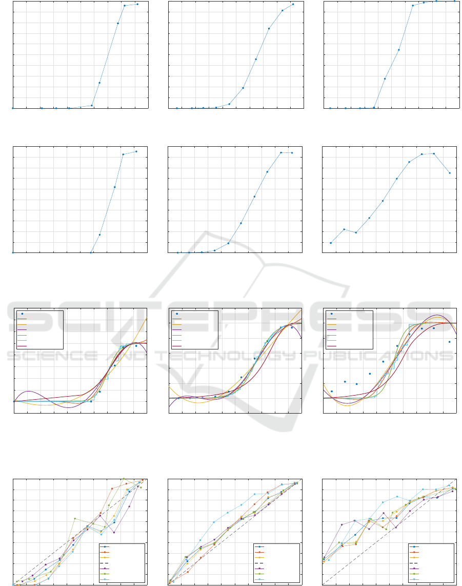
In Figure 1 we show the reliability diagrams for train-

ing and test set for the three datasets. The binning

has been performed with 10 uniformly-spaced bins, a

common strategy in related works. In all cases, the

trend is way far from the y = x diagonal line: a clear

sign that the classiﬁer is not well-calibrated. By con-

sidering the ADULT dataset (training set) as an exam-

ple, it is possible to see that all points whose score is

less than 0.7 lie below the y = x line: this means that

all points with score (as returned by SVM) less than or

equal to 0.7 have probability to belong to class 1 way

inferior with respect to the score itself; similarly, for

all points with score greater than 0.7, the true proba-

bility to belong to class 1 is superior with respect to

the score assigned by the classiﬁer.

Figure 2 shows the results in terms of ﬁtted curves

over the reliability diagram on the test set for the three

considered datasets. Conversely, in Figure 3 we show

the reliability diagram after calibration. For ease of

comparison, in Tables 1 and 2 we show the two ﬁg-

ure of merits (Brier score and Log-Loss score, respec-

tively) on both the training set and test set.

By considering the performances on test set, it

is possible to see that the three alternative methods

(Poly3, Poly4, NCS) have Brier score comparable to

state-of-the-art techniques (PS, IR, SC): Poly4 is the

best method for ABALONE, Poly3 and Poly4 equally

outperform other methods for ADULT and Poly3 is the

best method for PCN. In terms of Log-Loss, PS is the

best method for ABALONE and ADULT, whereas SC

is the best for PCN. Furthermore, the three alterna-

tive methods are featured by a lower computational

burden, being a plain curve ﬁtting over the reliability

diagram.

4 CONCLUSIONS

In this paper we reviewed three state-of-the-art tech-

niques for calibrating a binary classiﬁer in order to

return reliable probability estimates on the resulting

predictions. The three techniques (PS, IR and SC)

have been benchmarked on two well-known datasets

(ABALONE and ADULT) and an additional dataset

(PCN) against three lightweight methods (Poly3,

Poly4 and NSC), which basically perform a plain

curve ﬁtting on the reliability diagram. Computa-

tional results show that the three methods are com-

parable in terms of Brier score and Log-Loss score

with respect to the three state-of-the-art approaches.

For these tests we used a SVM classiﬁer due to its

uncalibrated behaviour and in order to stress the com-

parison amongst calibration techniques rather than

classiﬁcation systems. Nonetheless, future research

endeavours will consider the application of such tech-

niques to different classiﬁcation systems.

Indeed this study is part of a wider project concern-

ing the design and implementation of a modelling and

recognition system of faults and outages occurring

in the real-world power grid managed by “Azienda

Comunale Energia e Ambiente” (ACEA) company in

Rome, Italy. The recognition system, based on a one-

class classiﬁcation approach as the main core of a

larger system (De Santis et al., 2015), has been devel-

oped within the “ACEA Smart Grids project”. A ﬁrst

task consists in modelling and recognizing faults in

the power grid within a Decision Support System that

provides support for the commanding and dispatching

system, aiming at the implementation of Condition

Based Maintenance programs. Another very impor-

tant task consists in extracting from the learned fault

classiﬁcation model useful information for program-

ming and control procedures, such as the estimation

NCTA 2019 - 11th International Conference on Neural Computation Theory and Applications

492

0 0.1 0.2 0.3 0.4 0.5 0.6 0.7 0.8 0.9 1

Mean predicted value (score)

0.1

0.2

0.3

0.4

0.5

0.6

0.7

0.8

0.9

Fraction of positive instances (empirical probabilities)

(a) ABALONE (training set)

0 0.1 0.2 0.3 0.4 0.5 0.6 0.7 0.8 0.9 1

Mean predicted value (score)

0.1

0.2

0.3

0.4

0.5

0.6

0.7

0.8

0.9

Fraction of positive instances (empirical probabilities)

(b) ADULT (training set)

0 0.1 0.2 0.3 0.4 0.5 0.6 0.7 0.8 0.9 1

Mean predicted value (score)

0.1

0.2

0.3

0.4

0.5

0.6

0.7

0.8

0.9

Fraction of positive instances (empirical probabilities)

0 0.1 0.2 0.3 0.4 0.5 0.6 0.7 0.8 0.9 1

Mean predicted value (score)

0.1

0.2

0.3

0.4

0.5

0.6

0.7

0.8

0.9

Fraction of positive instances (empirical probabilities)

(d) ABALONE (test set)

0 0.1 0.2 0.3 0.4 0.5 0.6 0.7 0.8 0.9 1

Mean predicted value (score)

0.1

0.2

0.3

0.4

0.5

0.6

0.7

0.8

0.9

Fraction of positive instances (empirical probabilities)

(e) ADULT (test set)

0 0.1 0.2 0.3 0.4 0.5 0.6 0.7 0.8 0.9 1

Mean predicted value (score)

0.1

0.2

0.3

0.4

0.5

0.6

0.7

0.8

0.9

Fraction of positive instances (empirical probabilities)

(f) PCN (test set)

Figure 1: Reliability Diagrams.

0 0.1 0.2 0.3 0.4 0.5 0.6 0.7 0.8 0.9 1

Mean predicted value (score)

-0.2

0.2

0.4

0.6

0.8

1.2

1.4

1.6

Fraction of positive instances (empirical probabilities)

Reliability Diagram

NCS

Poly3

Poly4

(a) ABALONE

0 0.1 0.2 0.3 0.4 0.5 0.6 0.7 0.8 0.9 1

Mean predicted value (score)

-0.2

0.2

0.4

0.6

0.8

1.2

Fraction of positive instances (empirical probabilities)

Reliability Diagram

NCS

Poly3

Poly4

(b) ADULT

0 0.1 0.2 0.3 0.4 0.5 0.6 0.7 0.8 0.9 1

Mean predicted value (score)

-0.2

0.2

0.4

0.6

0.8

1.2

Fraction of positive instances (empirical probabilities)

Reliability Diagram

NCS

Poly3

Poly4

Figure 2: Reliability Diagrams vs. ﬁtted curves. For ABALONE we observe that for x ∈ (0,0.6) blue asterisks are missing,

meaning that there are no scores in such bins.

0 0.1 0.2 0.3 0.4 0.5 0.6 0.7 0.8 0.9 1

Mean predicted value (score)

0.1

0.2

0.3

0.4

0.5

0.6

0.7

0.8

0.9

Fraction of positive instances (empirical probabilities)

NCS

Poly3

Poly4

Perfect Calibration

(a) ABALONE

0 0.1 0.2 0.3 0.4 0.5 0.6 0.7 0.8 0.9 1

Mean predicted value (score)

0.1

0.2

0.3

0.4

0.5

0.6

0.7

0.8

0.9

Fraction of positive instances (empirical probabilities)

NCS

Poly3

Poly4

Perfect Calibration

(b) ADULT

0 0.1 0.2 0.3 0.4 0.5 0.6 0.7 0.8 0.9 1

Mean predicted value (score)

0.1

0.2

0.3

0.4

0.5

0.6

0.7

0.8

0.9

Fraction of positive instances (empirical probabilities)

NCS

Poly3

Poly4

Perfect Calibration

Figure 3: Reliability Diagrams after Calibration.

Calibration Techniques for Binary Classiﬁcation Problems: A Comparative Analysis

493

Table 1: Brier Score.

Method Abalone Adult PCN

Training Set Test Set Training Set Test Set Training Set Test Set

uncalibrated 0.1788 0.1911 0.2028 0.1754 0.1302 0.1814

PS 0.1140 0.1209 0.1057 0.1084 0.0488 0.1977

IR 0.1083 0.1215 0.1050 0.1081 0.0442 0.1934

SC 0.1189 0.1263 0.1143 0.1179 0.0767 0.2073

Poly3 0.1368 0.1355 0.1095 0.1069 0.0582 0.1822

Poly4 0.1172 0.1236 0.1059 0.1069 0.0579 0.1847

NCS 0.1142 0.1207 0.1057 0.1070 0.0493 0.1878

Table 2: Log-Loss Score.

Method Abalone Adult PCN

Training Set Test Set Training Set Test Set Training Set Test Set

uncalibrated 0.5293 0.550 0.5919 0.5306 0.4404 0.5508

PS 0.3711 0.3901 0.3301 0.3395 0.1716 0.8451

IR 0.3503 0.3943 0.3274 0.3453 0.1476 2.3263

SC 0.3938 0.4080 0.3573 0.3626 0.2867 0.6486

Poly3 0.4572 0.4586 0.3613 0.3807 0.2260 1.8316

Poly4 0.3865 0.4184 0.3660 0.4416 0.2245 1.7577

NCS 0.3865 0.3909 0.3406 0.3718 0.1843 2.0713

of the ﬁnancial risk associated to a set of power grid

states and network resilience analysis. When dealing

with risk assessment and cost beneﬁt analysis for net-

work expansion and maintenance planning, the avail-

ability of reliable probability estimates is of utmost

importance.

REFERENCES

Ayer, M., Brunk, H. D., Ewing, G. M., Reid, W. T., and

Silverman, E. (1955). An empirical distribution func-

tion for sampling with incomplete information. The

Annals of Mathematical Statistics, 26(4):641–647.

Berman, H. M., Westbrook, J., Feng, Z., Gilliland, G., Bhat,

T., Weissig, H., Shindyalov, I. N., and Bourne, P. E.

(2000). The protein data bank. Nucleic Acids Re-

search, 28(1):235–242.

Boser, B. E., Guyon, I., and Vapnik, V. (1992). A training

algorithm for optimal margin classiﬁers. In Proceed-

ings of the ﬁfth annual workshop on Computational

learning theory, pages 144–152. ACM.

Brier, G. W. (1950). Veriﬁcation of forecast expressed

in terms of probability. Monthly Weather Review,

78(1):1–3.

Butler, S. (2016). Algebraic aspects of the normalized

Laplacian, pages 295–315. Springer International

Publishing, Cham.

Cortes, C. and Vapnik, V. (1995). Support-vector networks.

Machine learning, 20(3):273–297.

Cristianini, N. and Shawe-Taylor, J. (2000). An Introduction

to Support Vector Machines and Other Kernel-based

Learning Methods. Cambridge University Press.

De Santis, E., Livi, L., Sadeghian, A., and Rizzi, A. (2015).

Modeling and recognition of smart grid faults by a

combined approach of dissimilarity learning and one-

class classiﬁcation. Neurocomputing, 170:368 – 383.

De Santis, E., Martino, A., Rizzi, A., and Frattale Mascioli,

F. M. (2018a). Dissimilarity space representations and

automatic feature selection for protein function pre-

diction. In 2018 International Joint Conference on

Neural Networks (IJCNN), pages 1–8.

De Santis, E., Paschero, M., Rizzi, A., and Frattale Mas-

cioli, F. M. (2018b). Evolutionary optimization of

an afﬁne model for vulnerability characterization in

smart grids. In 2018 International Joint Conference

on Neural Networks (IJCNN), pages 1–8.

DeGroot, M. H. and Fienberg, S. E. (1983). The com-

parison and evaluation of forecasters. Journal of the

Royal Statistical Society. Series D (The Statistician),

32(1/2):12–22.

Di Noia, A., Martino, A., Montanari, P., and Rizzi, A.

(2019). Supervised machine learning techniques and

genetic optimization for occupational diseases risk

prediction. Soft Computing.

Di Paola, L., De Ruvo, M., Paci, P., Santoni, D., and

Giuliani, A. (2012). Protein contact networks: an

emerging paradigm in chemistry. Chemical Reviews,

113(3):1598–1613.

Domingos, P. M. and Pazzani, M. J. (1996). Beyond inde-

pendence: Conditions for the optimality of the simple

bayesian classiﬁer. In Proceedings of the Thirteenth

NCTA 2019 - 11th International Conference on Neural Computation Theory and Applications

494

International Conference on International Conference

on Machine Learning, ICML’96, pages 105–112, San

Francisco, USA. Morgan Kaufmann Publishers Inc.

Dua, D. and Graff, C. (2019). UCI machine learning repos-

itory. http://archive.ics.uci.edu/ml.

Freedman, D. and Diaconis, P. (1981). On the histogram

as a density estimator: L2 theory. Zeitschrift f

Wahrscheinlichkeitstheorie und Verwandte Gebiete,

57(4):453–476.

Hastie, T., Tibshirani, R., and Friedman, J. (2001). The

elements of statistical learning. Springer-Verlag, New

York, USA.

Jain, A. K., Murty, M. N., and Flynn, P. J. (1999). Data

clustering: a review. ACM computing surveys (CSUR),

31(3):264–323.

Li, Y. H., Xu, J. Y., Tao, L., Li, X. F., Li, S., Zeng, X.,

Chen, S. Y., Zhang, P., Qin, C., Zhang, C., Chen, Z.,

Zhu, F., and Chen, Y. Z. (2016). Svm-prot 2016: A

web-server for machine learning prediction of protein

functional families from sequence irrespective of sim-

ilarity. PLOS ONE, 11(8):1–14.

Lin, H.-T., Lin, C.-J., and Weng, R. C. (2007). A note

on platt’s probabilistic outputs for support vector ma-

chines. Machine Learning, 68(3):267–276.

Lucena, B. (2018). Spline-based probability calibration.

arXiv preprint arXiv:1809.07751.

Maiorino, E., Rizzi, A., Sadeghian, A., and Giuliani, A.

(2017). Spectral reconstruction of protein contact net-

works. Physica A: Statistical Mechanics and its Ap-

plications, 471:804 – 817.

Martino, A., Giuliani, A., and Rizzi, A. (2018a). Gran-

ular computing techniques for bioinformatics pat-

tern recognition problems in non-metric spaces. In

Pedrycz, W. and Chen, S.-M., editors, Computational

Intelligence for Pattern Recognition, pages 53–81.

Springer International Publishing, Cham.

Martino, A., Maiorino, E., Giuliani, A., Giampieri, M., and

Rizzi, A. (2017a). Supervised approaches for function

prediction of proteins contact networks from topolog-

ical structure information. In Sharma, P. and Bianchi,

F. M., editors, Image Analysis, pages 285–296, Cham.

Springer International Publishing.

Martino, A., Rizzi, A., and Frattale Mascioli, F. M. (2017b).

Efﬁcient approaches for solving the large-scale k-

medoids problem. In Proceedings of the 9th Inter-

national Joint Conference on Computational Intelli-

gence - Volume 1: IJCCI,, pages 338–347. INSTICC,

SciTePress.

Martino, A., Rizzi, A., and Frattale Mascioli, F. M. (2018b).

Distance matrix pre-caching and distributed computa-

tion of internal validation indices in k-medoids clus-

tering. In 2018 International Joint Conference on

Neural Networks (IJCNN), pages 1–8.

Martino, A., Rizzi, A., and Frattale Mascioli, F. M. (2018c).

Supervised approaches for protein function prediction

by topological data analysis. In 2018 International

Joint Conference on Neural Networks (IJCNN), pages

1–8.

Martino, A., Rizzi, A., and Frattale Mascioli, F. M.

(2019). Efﬁcient approaches for solving the large-

scale k-medoids problem: Towards structured data.

In Sabourin, C., Merelo, J. J., Madani, K., and War-

wick, K., editors, Computational Intelligence: 9th In-

ternational Joint Conference, IJCCI 2017 Funchal-

Madeira, Portugal, November 1-3, 2017 Revised Se-

lected Papers, pages 199–219. Springer International

Publishing, Cham.

Minneci, F., Piovesan, D., Cozzetto, D., and Jones, D. T.

(2013). Ffpred 2.0: Improved homology-independent

prediction of gene ontology terms for eukaryotic pro-

tein sequences. PLOS ONE, 8(5):1–10.

Murphy, A. H. and Winkler, R. L. (1977). Reliability of sub-

jective probability forecasts of precipitation and tem-

perature. Journal of the Royal Statistical Society. Se-

ries C (Applied Statistics), 26(1):41–47.

Naeini, M. P., Cooper, G. F., and Hauskrecht, M. (2015).

Obtaining well calibrated probabilities using bayesian

binning. In Proceedings of the Twenty-Ninth AAAI

Conference on Artiﬁcial Intelligence, AAAI’15, pages

2901–2907. AAAI Press.

Niculescu-Mizil, A. and Caruana, R. (2005). Predicting

good probabilities with supervised learning. In Pro-

ceedings of the 22nd international conference on Ma-

chine learning, pages 625–632. ACM.

Parzen, E. (1962). On estimation of a probability den-

sity function and mode. The Annals of Mathematical

Statistics, 33(3):1065–1076.

Platt, J. (2000). Probabilities for sv machines. In Smola,

A. J., Bartlett, P., Sch

olkopf, B., and Schuurmans, D.,

editors, Advances in large margin classiﬁers, pages

61–74. MIT Press, Cambridge, MA, USA.

Sch

olkopf, B. and Smola, A. J. (2002). Learning with ker-

nels: support vector machines, regularization, opti-

mization, and beyond. MIT Press.

Scott, D. W. (1979). On optimal and data-based histograms.

Biometrika, 66(3):605–610.

Sturges, H. A. (1926). The choice of a class inter-

val. Journal of the American Statistical Association,

21(153):65–66.

The UniProt Consortium (2017). Uniprot: the univer-

sal protein knowledgebase. Nucleic Acids Research,

45(D1):D158–D169.

Wahba, G. (1990). Spline models for observational data,

volume 59. Siam.

Webb, E. C. (1992). Enzyme nomenclature 1992. Recom-

mendations of the Nomenclature Committee of the In-

ternational Union of Biochemistry and Molecular Bi-

ology on the Nomenclature and Classiﬁcation of En-

zymes. Academic Press, 6 edition.

Zadrozny, B. and Elkan, C. (2001). Obtaining calibrated

probability estimates from decision trees and naive

bayesian classiﬁers. In Proceedings of the Eigh-

teenth International Conference on Machine Learn-

ing, ICML ’01, pages 609–616, San Francisco, CA,

USA. Morgan Kaufmann Publishers Inc.

Zadrozny, B. and Elkan, C. (2002). Transforming classiﬁer

scores into accurate multiclass probability estimates.

In Proceedings of the eighth ACM SIGKDD interna-

tional conference on Knowledge discovery and data

mining, pages 694–699. ACM.

Calibration Techniques for Binary Classiﬁcation Problems: A Comparative Analysis

495