Vision based Indoor Obstacle Avoidance using a

Deep Convolutional Neural Network

Mohammad O. Khan and Gary B. Parker

Department of Computer Science, Connecticut College, New London, CT, U.S.A.

Keywords: Deep Learning, Artificial Neural Networks, Obstacle Avoidance, Indoor, TurtleBot, Mobile Robotics.

Abstract: A robust obstacle avoidance control program was developed for a mobile robot in the context of tight, dynamic

indoor environments. Deep Learning was applied in order to produce a refined classifier for decision making.

The network was trained on low quality raw RGB images. A fine-tuning approach was taken in order to

leverage pre-learned parameters from another network and to speed up learning time. The robot successfully

learned to avoid obstacles as it drove autonomously in a tight classroom/laboratory setting.

1 INTRODUCTION

The field of Deep Learning consists of algorithms that

learn using massive artificial neural network

architectures. Most Deep Learning models are built

with the intent of processing images. Some of these

architectures are capable of outperforming humans in

tasks like classifying objects, which simply means

differentiating one object from other objects (dog vs.

wolf, e.g.). In this paper, we present an application of

Deep Learning to the concept of autonomous driving

for a TurtleBot type robot within a tight

classroom/laboratory setting based strictly on images.

The robot was able to successfully and autonomously

drive without hitting obstacles within the

environment.

Krizhevsky, Sutskever, and Hinton (2012) put

forth a foundational paper in regards to Deep

Learning. They developed a neural network with 60

million parameters and 650,000 neurons. This

network had 5 convolutional layers along with a few

pooling layers and 3 fully connected layers including

a final output layer of 1000 outputs. At the time, they

achieved a top-5 classification (of the 1000 classes)

error rate of only 15.3% compared to a much higher

second-place error rate of 26.2%. This paper

contributed to the discussion of the importance of

depth in neural networks by noting that removal of a

single hidden layer dropped the top-1 classification

error rate by 2%.

http://cs.conncoll.edu/parker

Szegedy et al. (2014) entered the ILSVRC

challenge with a 22 layer deep network nicknamed

GoogLeNet – in part because most of the engineers

and research scientists on the team worked for Google

at the time. The team won the competition with 12

times fewer parameters than Krizhevsky’s deep

network and obtained an impressive 6.66% error rate

for top-5 classification. Following the pattern of

improvements, He, Zhang, Ren, and Sun (2015) of

Microsoft Research used a 19 layer deep neural

network for the task and obtained an accuracy of

4.94% for top-5 classification. This was a landmark

accomplishment as it is purported to be the first to

beat human level performance (5.1%) for the

ImageNet dataset.

The most relevant dataset to our research is that of

CIFAR10 from the Canadian Institute for Advanced

Research (Krizhevsky, 2009b). Alex Krizhevsky

outlined the use of this dataset when he developed it

in 2009 for his Master’s Thesis during his time at the

University of Toronto (2009a). Prior to this, tiny

images on the scale of 32 x 32 were not easily labeled

for classification tasks in regards to algorithms like

Deep Learning. The CIFAR10 dataset includes 10

different classes: airplane, automobile, bird, cat, deer,

dog, frog, horse, ship, and truck. The classes are set

up in a way to be mutually exclusive. For example,

automobile and truck are completely different

categories. Krizhevsky developed different deep

neural network models in 2010 to run training with

the dataset. At the time he obtained the highest

Khan, M. and Parker, G.

Vision based Indoor Obstacle Avoidance using a Deep Convolutional Neural Network.

DOI: 10.5220/0008165104030411

In Proceedings of the 11th International Joint Conference on Computational Intelligence (IJCCI 2019), pages 403-411

ISBN: 978-989-758-384-1

403

accuracy using this dataset as his best model

classified objects correctly with a success rate of

78.9% (Krizhevsky, 2010). Since then, Mishkin and

Matas (2016) have obtained 94.16% accuracy on the

CIFAR10 dataset. Whereas, Springenberg et al.

(2015) have obtained 95.59% accuracy and the

current best performance is by Graham (2014) with

an accuracy of 96.53% using max pooling.

There has been strong interest in using the

TurtleBot platform for obstacle detection and

avoidance. Boucher (2012) used the Point Cloud

Library and depth information along with plane

detection algorithms to build methods of obstacle

avoidance. High curvature edge detection was used to

locate boundaries between the ground and objects that

rest on the ground. Other researchers have considered

the use of Deep Learning for the purpose of obstacle

avoidance using the TurtleBot platform.

Tai, Li, and Liu (2016) used depth images as the

only input into the deep network for training

purposes. They discretized control commands with

outputs such as: “go-straightforward”, “turning-half-

right”, “turning-full-right”, etc. The depth image was

from a Kinect camera with dimensions of 640 x 480.

This image was downsampled to 160 x 120. Three

stages of processing were done where the layering

was ordered as such: convolution, activation, pooling.

The first convolution layer used 32 convolution

kernels, each of size 5 x 5. The final layer included a

fully-connected layer with outputs for each

discretized movement decision. In all trials, the robot

never collided with obstacles, and the accuracy

obtained after training in relation to the testing set was

80.2%. Their network was trained only on 1104 depth

images. The environment used in this dataset seems

fairly straightforward – meaning that the only

“obstacles” seems to be walls or pillars. The

environment was not dynamic. Tai and Liu (2016)

produced another paper related to the previous paper.

Instead of a real-world environment, this was tested

in a simulated environment provided by the TurtleBot

platform, called Gazebo. Different types of corridor

environments were tested and learned. A

reinforcement learning technique called Q-learning

was paired with the power of Deep Learning. The

robot, once again, used depth images and the training

was done using Caffe. Other deep reinforcement

learning research included real-world evaluation on a

TurtleBot (Tai et al., 2017), using dueling deep

double Q networks trained to learn obstacle

avoidance (Xie et al., 2017), and using a fully

connected NN to map to Q-values for obstacle

avoidance (Wu et al., 2019).

Tai, Li, and Liu (2017) applied Deep Learning

using several convolutional neural network layers to

process depth images in order to learn obstacle

avoidance for a TurtleBot in the real world. This is

very similar to our work, except they used depth

images, the obstacles were just a corridor, and they

train from scratch instead of using transfer learning as

we did.

Our research provides a distinctive approach in

comparison to these works. Research like Boucher’s

does not consider higher level learning, but instead

builds upon advanced expert systems, which can

detect differentials in the ground plane. By focusing

on Deep Learning, our research allows a pattern based

learning approach that is more general and one which

does not need to be explicitly programmed. While Tai

et al. used Deep Learning, their dataset was limited

with just over 1100 images. We built our own dataset

to have over 30,000 images, increasing the size of the

effective dataset by about 28 times. The environment

for our research is more complex than just the flat

surfaces of walls and columns. As in Xie’s work, in

our research the learning was done on a dataset that

was based on raw monocular RGB images. This

opens the door to further research with cameras that

do not have depth. Moreover, the sizes of the images

used in our research were dramatically smaller, which

also opens up the door for faster training and a speed

up in forward propagation. Lastly, similar to a few of

these works, the results of our work were tested in the

real world as opposed to a simulated environment.

2 DEEP LEARNING

Consider a standard feed-forward artificial neural

network that is fully connected between each layer

being used to process a 100 x 100 pixel image. With

3 color channels, we would have 100 x 100 x 3 or

30,000 inputs to our neural network. This is a large

number of inputs for a standard neural network to

process. Deep Learning directly addresses this

limitation.

The convolution layer passes convolution

windows over the image to produce new images that

are smaller. The number of images produced can be

specified by the programmer. Each new image will be

accompanied by a convolution kernel signifying the

weights. Instead of sending all input values from layer

to layer, deep networks are designed to take regions

or subsamples of inputs. For images this means that

instead of sending all pixels in the entire image as

inputs, different neurons will only take regions of the

image as inputs – full connectivity is reduced to local

NCTA 2019 - 11th International Conference on Neural Computation Theory and Applications

404

connectivity. We take an image and extract local

regions of depth 3 for the color channels along with

their respective pixel values and input them into a

neuron. Supposing that our local receptive fields are

of size 5 x 5, this neuron takes in an input of

dimensions 5 x 5 x 3 for that particular portion of the

3 color channel image. The local receptive fields can

be seen as small windows that slide over our image,

where the number of panes on the window is

predefined. These panes help determine what features

under the window we want to extract, and over time

these features are better refined. The weighted

windows are commonly called kernels. Depending on

the type of kernel, different features of the image may

be highlighted, such as blurring and sharpening. In

this way, networks can develop identification of

complex patterns in datasets just by applying kernel

filters. Deep networks develop these kernels through

training without being explicitly programmed to do

so. The only supervision is from a loss function in the

output layer denoting how close the network’s

prediction was to the actual value of the image.

Through training, these kernels become more fine-

grained to reduce the loss function’s output.

Pooling is applied to each one of the convolution

images. Deep networks are stacked in such a way as

to include many different types of layers. A general

strategy is to follow a convolution layer with a type

of layer called a pooling layer. The convolution layer

is responsible for learning the lower level features of

an image, such as edges. The pooling layer seeks to

detect a higher level understanding of the lower level

features from the convolution layers. Pooling is also

good for building invariance to local translations.

This means that even if the input region is slightly

translated, most of the pooled output values will not

change. By employing max pooling (defined below),

dominant features, or regions with the largest values,

can be extracted and fed into later layers of the

network. Along with this benefit, the image is also

reduced dramatically because it is downsampled in

one of three ways:

1) Max pooling – The maximum pixel value is

chosen out of a rectangular region of pixels.

2) Min pooling – The minimum pixel value is chosen

out of a rectangular region of pixels.

3) Average pooling – The average pixel value is

chosen out of a rectangular region of pixels.

Reducing the size of the image dramatically cuts

down on the amount of processing needed to train the

higher level features of the network. In terms of

processing, the idea is similar to convolution as we

still pass a window over our image.

Convolution and pooling dominate the discussion

about types of network layers. However, there are a

few other types of layers that were used in this

research.

The Rectified Linear Unit (RLU) layer

(Krizhevsky et al., 2012) has recently grown in

popularity. Many researchers consider this over using

the sigmoid activation function. In fact, they were

able to accelerate convergence in their training by a

factor of 6 times in relation to the sigmoid activation

function using this function. This is a fairly

straightforward operation: the function takes a

numerical input X and returns it if it is positive,

otherwise it returns -1 * X. This effectively eliminates

negative inputs and boosts computation time since

complex computations such as exponentiation are not

needed.

The Local Response Normalization layer

(Krizhevsky et al., 2012) imitates biological lateral

inhibition – excited neurons have the capability of

subduing neighbor neurons. A neural “message” is

amplified and focused by this differential in neuron

excitement. These layers allow neuron’s with large

activation values to be much more influential than

other neurons. Following the pattern of feature

recognition in every layer, these layers allow

significant features to “survive” deeper into the

network.

The fully connected layer, which is like any

regular multi-layered perceptron, is generally the

final layer if it’s used in a network. The outputs of the

neurons in this layer are the actual outputs of the

network. Connected to this layer is the loss layer

where the network compares desired outputs to actual

outputs, and the learning is initiated here in terms of

gradient descent updates.

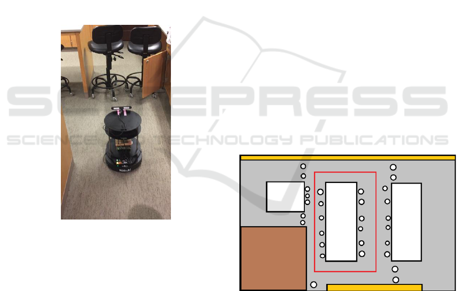
3 THE ROBOT

The robot used for this research (Figure 1) was the

“Deep Learning Robot” from Autonomous. Its basic

functionality is essentially equivalent to that of the

TurtleBot platform. The robot includes an Asus Xtion

Pro 3D Depth Camera, a microphone embedded in the

camera, and a speaker. A Kobuki mobile base allows

it to rotate and move in any direction on the ground

plane. Most importantly, it is equipped with an Nvidia

Tegra TK1, which allows us to carry out Deep

Learning computations on a GPU instead of having to

resort to extremely long wait times for training with a

CPU. This is its main difference from a regular

TurtleBot. While the Tegra TK1 is a powerful mobile

processor, it only has 2GB of memory. This is

Vision based Indoor Obstacle Avoidance using a Deep Convolutional Neural Network

405

problematic for training very deep networks because

holding too many parameters in memory causes the

robot to crash. While training, the robot is unstable

because of this limited memory so running multiple

programs at the same time is to be avoided.

The robot comes equipped with the Deep

Learning frameworks of Google TensorFlow, Torch,

Theano, and Caffe (we used Caffe), and CUDA and

cuDNN are provided for implementing Deep

Learning on GPUs and for speeding up that

computation. This robot is virtually a computer in

itself, and it allows us to treat it as such as it is very

compatible with Ubuntu 14.04. The TurtleBot

framework works hand in hand with the Robot

Operating System (ROS), which is used to control the

robot and to have access to all information coming

from any of the robot’s sensors. ROS is an “open-

source, meta-operating system” which allows

hardware abstraction, low-level control and message

passing between different modules/processes.

Figure 1: Photograph of the Deep Learning Robot.

4 OBSTACLE AVOIDANCE

The problem scenario is that of training a deep neural

network to learn autonomous driving of a vehicle in a

tight, chaotic room/office environment. To test the

functionality and success of the program, the

performance of the robot was compared to the end

goals. The end goals are primarily that the TurtleBot

should autonomously follow an approximately

rectangular path in a tight environment without

colliding into obstacles. A description of this

environment is provided below.

4.1 Environment

The Robotics Lab with obstacles in the room provides

a reasonably complex environment for our tests.

Figure 2 demonstrates this approximate environment

set up. The approximate rectangular path that was

configured was the perimeter of a long lab table. This

table only has 3 planes of support on the underside;

otherwise there are gaps underneath the table. White

rectangles with dark borders are lab tables. The north

and south sides of the tables are solid (2 of the planes

of support), whereas the east and west sides have

gaps. The gap size is large enough for the robot to be

able to drive through, but chairs (white circles with

dark borders) were placed in those locations. The total

radii of the chairs are larger than the circles shown

because the feet of the chairs extend out further.

There is no gap for the robot to move in between

neighbouring chairs (in most cases). The dark brown

rectangle (southwest corner of the lab) is a colony

space – boxed off area of the lab that may be used for

other experiments, but there are borders (one foot

high solid walls) that the robot would need to avoid

hitting. The golden rectangles (north and south walls

of the lab) denote cabinets which the robot must also

avoid. The red rectangle in the middle of the figure

shows the path around the center table that the robot

must follow or the general path it needs to go in on its

way as it avoids chairs, tables, boxes, etc. In separate

runs this path must be completed in both clockwise

and counter clockwise directions.

Figure 2: A visual of the environment with lab tables,

chairs, and cabinets. Images are provided below to help

understand this environment even more. The top of the

drawing is approximately north.

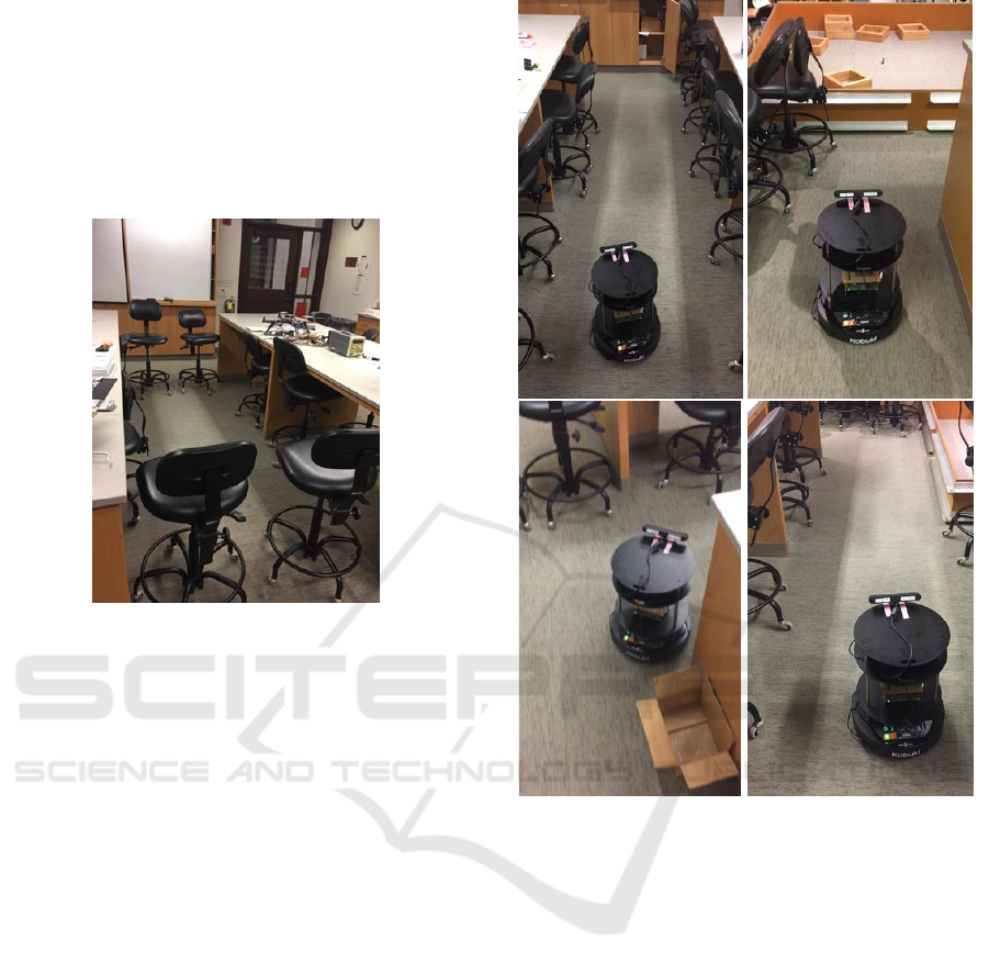
One can see from Figure 3 that the gaps were

closed with moveable round chairs. Each chair has 5

rounded legs and a circular stump. The chair heights

can be adjusted and the orientation can change 360

degrees for both the base and the actual seating.

Sample images are provided in the Figures 1, 3, and

NCTA 2019 - 11th International Conference on Neural Computation Theory and Applications

406

4 to visualize different possible orientations for the

chairs. These were chosen as the main objects of

interest because they are not solid – there is clearly a

good amount of gap area in between the legs. This

allows for complexity in defining what an obstacle is

and what and obstacle is not. The robot must not

simply learn to follow the color of the carpet because

even the gaps reveal the carpet.

Figure 3: Photograph showing chairs and spacing.

The camera for the robot faces down at about 40

degrees from the vertical position, so it is important

to design an environment that is complex enough, in

terms of objects close to the ground, to be a problem

of interest. To highlight the point of this experiment,

if the environment was built only using cardboard or

other flat material as the main obstacle in the

environment, then there would be a fairly

straightforward solution. There would not be much

variety, apart from lighting conditions, as to what

material needed to be avoided. By using the chairs,

the environment was more natural and complex. Not

only were the chairs not solid surfaces, they were

typically moved by students overnight. While they

might be in the same relative location, the orientations

were completely different each time. This adds

complexity to the problem because it is not easy for a

pattern to be developed since the orientation keeps

changing. This means that for obstacle avoidance to

be successful the deep neural network necessarily

needs to develop an “understanding” that chairs are to

be avoided. With enough gaps in between chairs and

the legs of the chairs having significant gaps, the

robot will still see the carpeted area. Thus, it cannot

just develop a control program to follow a carpeted

area, but instead needs a more complex pattern to be

recognized from the dataset.

Figure 4: The images above demonstrate various obstacle

avoidance scenarios.

It is important to establish guidelines as far as

environmental set up because there may be scenarios

that are impossible for the robot to solve. In our

research, we dealt with two. In the first, if there is

enough of a gap between two chairs the robot may

make the decision to go straight instead of turning

away from the chairs. In the second, if the robot is

facing a cabinet directly head on. Even for a human

with limited peripheral vision, it would be impossible

to know which direction to turn. There is no way to

have metaknowledge about which direction contains

an obstacle and which does not. This is not a fair

scenario to include in the dataset. To solve the former

of the two issues, the environment included chairs

that were placed close enough to have a small enough

gap that the robot would not be able to fit through. To

solve the latter of the two scenarios, cabineted areas

included an open cabinet that swivelled to a direction

the robot was supposed to avoid. Not only does this

Vision based Indoor Obstacle Avoidance using a Deep Convolutional Neural Network

407

add more chaos to the environment (there are various

different items in the cabinets which adds to the

complexity of developing a pattern), but it also

establishes rough guidelines as to the correct path.

Chairs, cabinets, and tables were not the only

obstacles to avoid. A few images in the dataset

included small cardboard boxes. A good amount of

the dataset included the borders of a colony space

environment. It was important to include obstacles

like this in order to confirm that the concept of

obstacle avoidance was being abstracted instead of

the robot only avoiding black colored objects (the

black chairs). It is also significant to note that students

used the lab throughout the day and night, so

conditions of the carpet changed while the dataset

was being developed. For example, coins were found

laid out on the ground near a turn in the path on one

day. On another day, shreds of paper were at different

locations on the path. We decided not to remove some

of these items while building the dataset because it

only adds to the diversity in what we might consider

edge cases.

4.2 Dataset Collection

During data collection the robot was controlled

remotely by a user on a keyboard (connected through

a computer on Bluetooth) as it was driven around the

lab following the path in both directions. The robot

maintained continuous forward movement as the

operator designated left, right, or straight. To increase

the diversity of the dataset, different starting points

were chosen and hard scenarios such as being close

to walls were considered. Overall, 30,754 images

were collected and labelled.

The script processed about 10 images per second,

but not every image was saved. While no time record

was kept, an estimated 1.5 – 2 hours were spent on

trial runs and collections. In the initial testing

conditions, we found that there were edge cases that

were missing, so more data was added over time. By

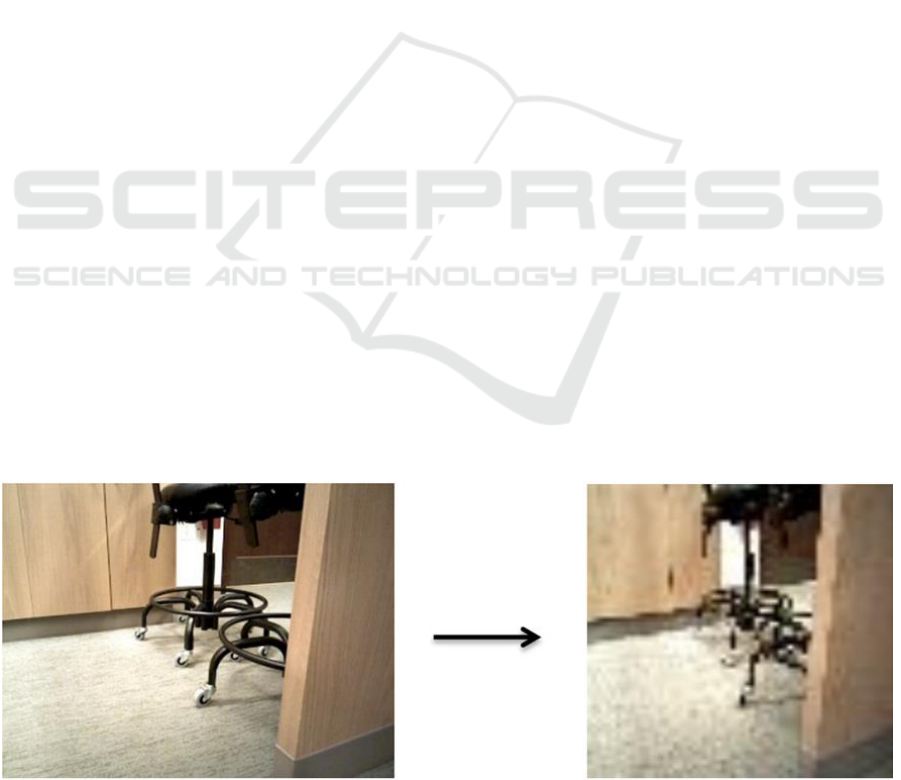
default, the images from the Asus Xtion Pro are of

dimension 640 x 480. While this would provide a

great amount of detail to train on, it would take an

incredible amount of processing power and time to

train to a significant accuracy. For our deep network

we downsample this image to 64 x 64 (Figure 5).

5 DEVELOPMENT OF DEEP

NEURAL NET ARCHITECTURE

We initially started by using an imitation of Alex

Krizhevsky’s deep network architecture to solve the

CIFAR10 dataset. The plan was to augment this

network with our own dataset. We obtained about

74% accuracy for that dataset. We took the weights

of the network from it having learned the CIFAR10

data, and then fine-tuned it for our own purpose –

obstacle avoidance while driving autonomously.

The thought for fine-tuning was inspired from the

notion that the lower level features detected by the

network are general enough to be applied to the

problem of obstacle detection. Intuitively, there is a

large difference between detecting an airplane and

detecting a dog or a cat. However, Krizhevsky’s

network is capable of differentiating between the two

based on the same kernel weights. That seems to be a

large area of coverage for the type of data provided.

The other thought here was that Krizhevsky’s

network was trained on 32 x 32 dimension images.

Since our images will be 64 x 64 pixels, we may

expect that there will be a boost in accuracy.

The complete network used for this research is

shown in Figure 6. It is split into three lines to

ease the visualization. We can see that there are 3

Figure 5: Reducing the image resolution from 640 x 480 to 64 x 64.

NCTA 2019 - 11th International Conference on Neural Computation Theory and Applications

408

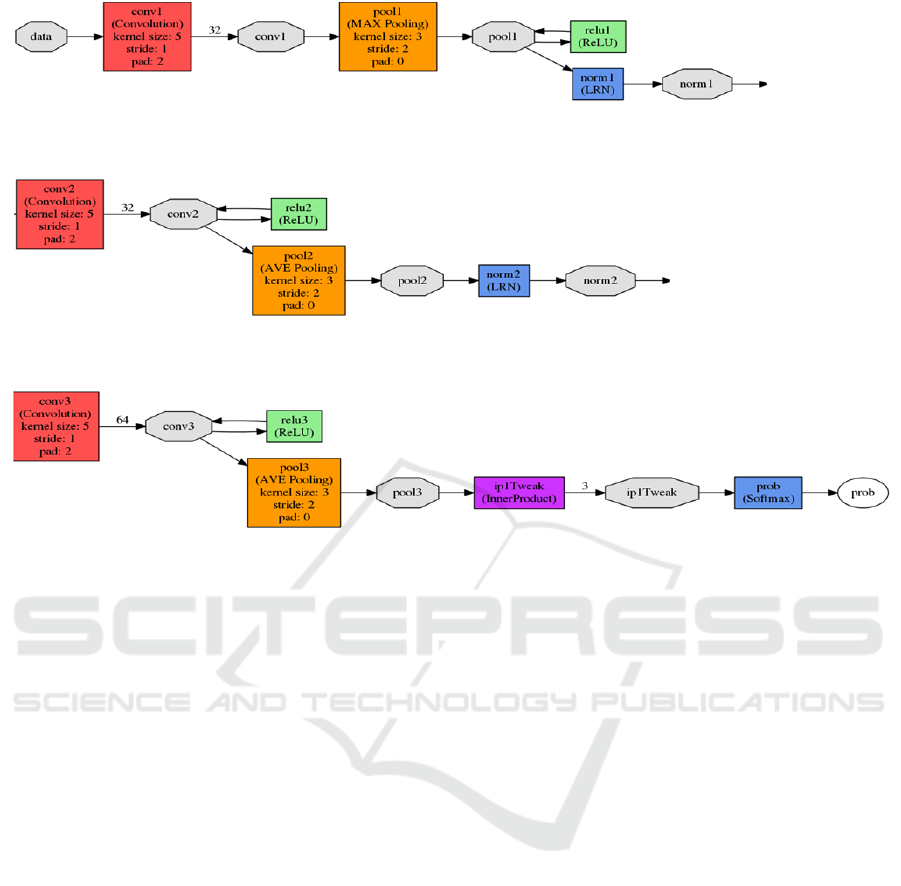
Figure 6: The final architecture for the deep network. This is inspired by the architecture for solving the CIFAR10 dataset.

The rectangles represent layers. The octagons represent data.

iterations of the layer combinations of convolution,

pooling, and normalization. Note that the fine-tuning

of the network is evident from the visual. The layer

“ip1Tweak” is labeled as such because the final layer

of Krizhevsky’s network was removed and replaced

with an inner product (“ip”), or also considered fully

connected, layer that only had 3 outputs. This is

signified by the value 3 above the ip1Tweak layer in

the visual. The 3 outputs correspond to the decision

making of the TurtleBot in terms of autonomous

driving directions. The original network included 32

convolution kernels for the first convolution, 32

convolution kernels for the second convolution, and

64 convolution kernels for the last one. We can also

see how each convolution layer is immediately

followed by a pooling layer. Every convolution layer

also includes a rectified linear unit attached to it.

Local Response Normalization also appears to be an

effective addition to this network, as it augments the

outputs of 2 of the 3 pooling layers. The dataset was

split as such for the final network: 23,065 images for

training and 7,689 images for testing – a 75% training

split of the entire dataset.

The hyperparameters were:

• testing iterations: 100; basically how many

forward passes the test will carry out.

• batch size: 77; this is for batch gradient descent

– notice that batch size * testing iterations will

cover the entire testing dataset.

• base learning rate: 0.001

• momentum: 0.9

• weight decay: 0.004

• learning rate policy: fixed

• maximum training iterations: 15,000

• testing interval: 150; testing will be carried out

every 150 training iterations.

These hyperparameters were determined through

several experiments in order to find the desired level

of accuracy and performance. Some of these

parameters are surely subjective. For example, we

considered testing interval to be much less than it

usually is for large networks (on the order of 1000).

The reason for making this a small value is so that we

can analyze shifts in learning in a decent amount of

time instead of having to wait for over half an hour.

The number of maximum iterations was chosen as an

estimation of the number of epochs the network may

have needed to stabilize. The batch size of the training

data is 77 images, thus we would need about 300

iterations to cover the whole training dataset. Hence,

the number for maximum iterations was established

as 15,000 in order for the network to go through about

50 epochs.

Vision based Indoor Obstacle Avoidance using a Deep Convolutional Neural Network

409

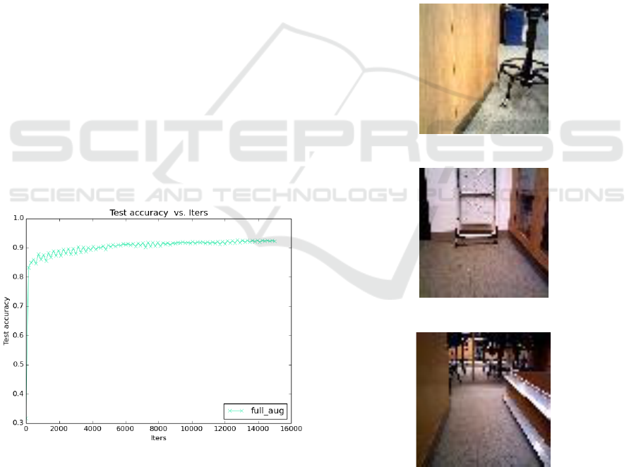
6 RESULTS FOR AUTONOMOUS

DRIVING

Starting with a Krizhevsky network trained on the

CIFAR10 dataset and replacing the final layer with a

tweaked fully connected layer, we ran the Deep

Learning neural network on 30,000 images generated

for the obstacle avoidance problem. The network was

able to obtain an accuracy of about 92% after 15,000

iterations (Figure 7). It took the network about 200

iterations to get to the 84% accuracy mark and around

2000 iterations to achieve an accuracy of 90%. Ten

different test runs in the actual environment were

completed where the robot was reversed after a

completion of a lap in order to complete the lap in the

both directions. The robot did, although rarely,

slightly graze against the leg of a chair or a cardboard

box. However, this did not change the trajectory of

the robot and it was still able to complete its course.

For this reason, these rare occurrences were not

considered as major events for hitting an obstacle.

One could argue that the turning angle for the

robot is the only issue here since this is such a tight

environment. Though the network made the right

decision, the movement of the physical robot may

have been slightly too much. This can be corrected

with very small tweaks in the values of turning radii

for the different decisions, however this does not

reflect on or add to the discussion about the

performance of the deep network in itself.

Figure 7: The performance of the network in relation to

iterations for the fine-tuned Krizhevsky network trained

with over 30,000 images. The first 15,000 iterations are

shown. It took about 200 iterations to get to the 84% mark

and by 15,000 it was at 92% accuracy.

6.1 Visual Analysis of Results

While observing the robot during particular situations

of interest we noted that it routinely performed the

correct action. The scenario of the open cabinet was

not a challenge for the robot (Figure 1 and Figure 4

top left). As previously mentioned, this helped

augment the robots path learning. We observed that

the robot was successfully able to navigate the tight

corridor and move away from chair obstacles (Figure

4 top images) and the border of the colony space,

which showed that the robot learned to avoid more

than just the chairs (Figure 4 right images). Although,

the cardboard box was seldom included in the original

training dataset, the robot clearly had pattern

recognition broad enough to be able to avoid it

(Figure 4 bottom left). Figure 8 shows three examples

of the output of the neural network.

left 0, straight 0, right 1

left 0.73, straight 0.27, right 0

left 0.02, straight 0.96, right 0.02

Figure 8: A sampling of scenarios where the neural network

made live decisions and the outputs of the NN are shown

for each (they will total 1.0). The NN will have the robot

turn right in the top scenario, left in the middle, and straight

in the bottom.

NCTA 2019 - 11th International Conference on Neural Computation Theory and Applications

410

7 CONCLUSIONS

The approach of fine-tuning Krizhevsky’s network

that solved the CIFAR10 dataset was highly

successful. The robot effectively avoided obstacles in

the original room where the dataset was collected.

The robot also avoided colliding into other obstacles

that were not part of the dataset – the deep network

did not solely focus on chairs and cabinets as the only

obstacles to avoid. In regard to accuracy, this

approach seems more successful than the previous

approaches that utilized depth. In the future, different

dimensions (other than 64x64) may be considered. It

would be valuable to potentially find a definable

relationship between the image dimension and

network accuracy.

REFERENCES

Boucher, S., 2012. Obstacle detection and avoidance using

TurtleBot platform and Xbox Kinect. Research

Assistantship Report. Department of Computer

Science, Rochester Institute of Technology.

Graham, B., 2014. Fractional max-pooling. CoRR,

arXiv:1412.6071.

He, K. , Zhang, X., Ren, S. & Sun, J., 2015. Delving deep

into rectifiers: Surpassing human level performance on

imagenet classification. Proceedings of the

International Conference on Computer Vision.

Krizhevsky, A., 2009a. Learning multiple layers of features

from tiny images. Master’s thesis, Department of

Computer Science, University of Toronto.

Krizhevsky, A., 2009b. CIFAR10 dataset project page:

https://www.cs.toronto.edu/~kriz/cifar.html

Krizhevsky, A., 2010. Convolutional deep belief networks

on CIFAR-10. Unpublished manuscript.

Krizhevsky, A, Sutskever, I. & Hinton, G., 2012. ImageNet

classification with deep convolutional neural networks.

Neural Information Processing Systems (NIPS).

Mishkin, D. & Matas, J., 2016. All you need is a good init.

Proceedings of the International Conference on

Learning Representations (ICLR).

Springenberg, J.T., Dosovitskiy, A., Brox, T., Riedmiller,

M., 2015. Striving for simplicity: the all convolutional

net. Proceedings of the International Conference on

Learning Representations (ICLR).

Szegedy, C., Liu, W., Jia, Y., Sermanet, P., Reed, S.,

Anguelov, D., Erhan, D., Vanhoucke,V., and

Rabinovich, A., 2014. Going deeper with convolutions.

Proceedings of the IEEE Conference on Computer

Vision and Pattern Recognition (CVPR).

Tai, L., Li, S. & Liu, M., 2016. A deep-network solution

towards modeless obstacle avoidance. Proceedings of

the IEEE/RSJ International Conference on Intelligent

Robots and Systems (IROS).

Tai, L. & Liu, M., 2016. A robot exploration strategy based

on q-learning network. Proceedings of the IEEE

International Conference on Real-time Computing and

Robotics (RCAR).

Tai, L., Li, S., Liu, M. 2017. Autonomous exploration of

mobile robots through deep neural networks.

International Journal of Advanced Robotic Systems.

Tai, L., Paolo, G., & Liu, M. 2017. Virtual-to-real deep

reinforcement learning: continuous control of mobile

robots for mapless navigation. Proceedings of the

IEEE/RSJ International Conference on Intelligent

Robots and Systems (IROS 2017).

Wu, K., Esfahani, M., Yuan, S., & Wang, H. 2019. Depth-

based obstacle avoidance through deep reinforcement

learning. Proceedings of the 5th International

Conference on Mechatronics and Robotics.

Xie, L., Wang, S., Markham, A., & Trigoni, N. 2017.

Towards monocular vision based obstacle avoidance

through deep reinforcement learning. Proceedings of

the RSS 2017 Workshop on New Frontiers for Deep

Learning in Robotics.

Vision based Indoor Obstacle Avoidance using a Deep Convolutional Neural Network

411