Learning Method of Recurrent Spiking Neural Networks to Realize

Various Firing Patterns using Particle Swarm Optimization

Yasuaki Kuroe

1,2

, Hitoshi Iima

and Yutaka Maeda

Faculty of Engineering Science, Kansai University, Suita-shi, Osaka, Japan

Faculty of Information and Human Sciences, Kyoto Institute of Technology, Kyoto, Japan

Keywords:

Spiking Neural Network, Learning Method, Particle Swarm Optimization, Burst Firing, Periodic Firing.

Abstract:

Recently it has been reported that artiﬁcial spiking neural networks (SNNs) are computationally more pow-

erful than the conventional neural networks. In biological neural networks of living organisms, various ﬁring

patterns of nerve cells have been observed, typical examples of which are burst ﬁrings and periodic ﬁrings. In

this paper we propose a learning method which can realize various ﬁring patterns for recurrent SNNs (RSSNs).

We have already proposed learning methods of RSNNs in which the learning problem is formulated such that

the number of spikes emitted by a neuron and their ﬁring instants coincide with given desired ones. In this

paper, in addition to that, we consider several desired properties of a target RSNN and proposes cost func-

tions for realizing them. Since the proposed cost functions are not differentiable with respect to the learning

parameters, we propose a learning method based on the particle swarm optimization.

1 INTRODUCTION

Recently there is a surge in the research of artiﬁ-

cial spiking neural networks (SNNs) due to the fact

that the functions of spiking neurons are closer to

the physiological functions of the generic biologi-

cal neurons than the conventional threshold and sig-

moidal neurons (Mass and Bishop C., 1998; Gerst-

ner and van Hemmen, 1993b; Mass, 1997b). In arti-

ﬁcial spiking neural networks the information is en-

coded and processed by the spike trains (sequence of

action potentials) similar to the biological neural net-

works (BNNs), through a discontinuous and nonlin-

ear encoding mechanism (Mass and Bishop C., 1998;

Gerstner and van Hemmen, 1993b). The conventional

neuron models usually tend to ignore these sophisti-

cated discontinuous encoding mechanisms. In addi-

tion to the SNNs’ similarity to the BNNs, recently it

has been reported that they are computationally more

powerful than the conventional artiﬁcial neural net-

works (Mass, 1997b; Mass, 1997a; Mass, 1996). It

is however much more difﬁcult to analyze and syn-

thesize the SNNs than the conventional threshold and

sigmoidal neural networks. This is due to their as-

sociated nonlinear and discontinuous encoding mech-

anisms, which make the SNNs continuous and dis-

crete hybrid-dynamical systems. In this paper we dis-

cuss a learning method, which is one of fundamental

problems of NNs, for the recurrent spiking neural net-

works (RSNNs).

In the case of the sigmoidal neural networks, the

backpropagation method was proposed by Rumelhart

et al. (Rumelhart and McClelland, 1986) for feed-

forward types of neural networks, which is one of

the pioneering works that trigger the research inter-

ests of applications of the neural networks. Following

the backpropagation method, learning methods have

been developed for recurrent sigmoidal neural net-

works (Kuroe, 1992).

In the case of the SNNs, their learning methods

have not been actively studied due to their associ-

ated nonlinear and discontinuous encoding mecha-

nisms and only a few studies have been done. As

unsupervised learning W. Gestner et al. proposed

a learning method for feedforward SNNs, which is

based on the concept of the Hebbian learning (Gerst-

ner and van Hemmen, 1993a). As supervised learning

for SNNs the following studies have been done. K.

Selvaratnam et al. proposed a gradient based learn-

ing method for RSNNs (Selvaratnam and Mori, 2000)

based on sensitivity equation approach and Y. Kuroe

et al. proposed based on adjoint equation approach

(Kuroe and Ueyama, 2010). Backpropagation-like

learning method is proposed for feedforward SNNs

(Bohte et al., 2002) and for deep SNNs (Lee and

Pfeiffer, 2016).

Kuroe, Y., Iima, H. and Maeda, Y.

Learning Method of Recurrent Spiking Neural Networks to Realize Various Firing Patterns using Particle Swarm Optimization.

DOI: 10.5220/0008164704790486

In Proceedings of the 11th International Joint Conference on Computational Intelligence (IJCCI 2019), pages 479-486

ISBN: 978-989-758-384-1

479

s+c





Membrane

Potential

Spike

Train

reset

Trigger

Summed

Potential

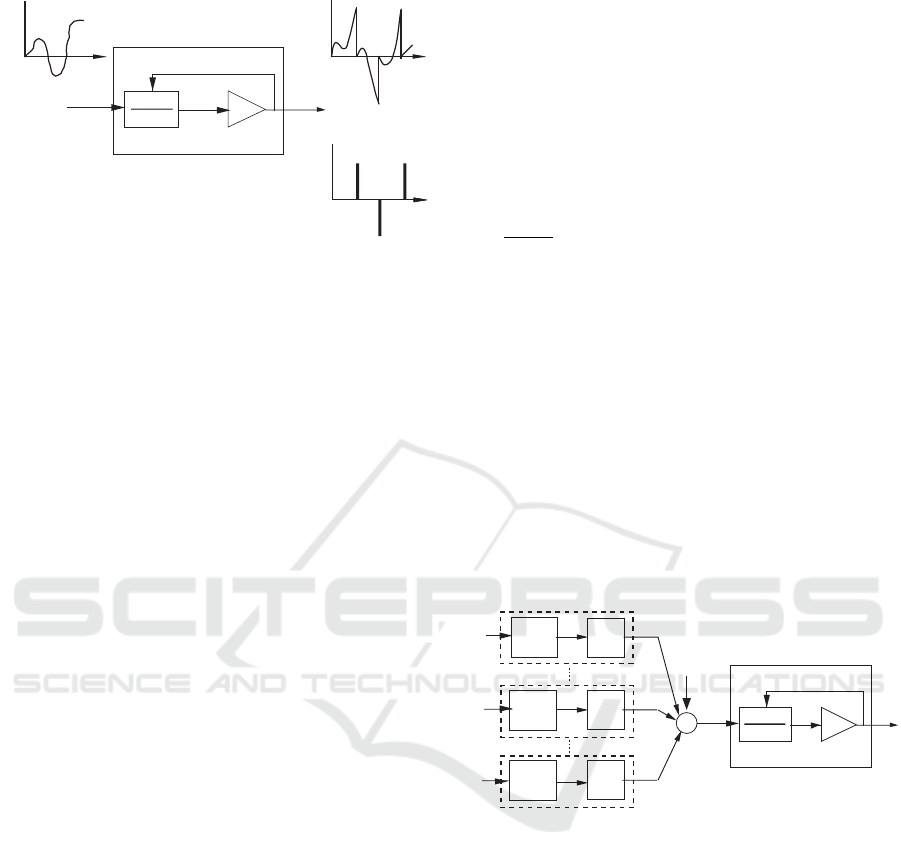
Figure 1: Schematic of the ﬁring mechanism of the integrate

and ﬁre type SN.

In biological neural networks of living organisms,

various ﬁring patterns of nerve cells have been ob-

served (Izhikevich, 2007), typical examples of which

are burst ﬁrings and periodic ﬁrings. It is expected

that artiﬁcial SNNs with recurrent architectures re-

alize various complicated ﬁring patterns (Izhikevich,

2004; Izhikevich, 2007) because of their behavior as

nonlinear dynamical systems. In this paper we pro-

pose a learning method which can realize various ﬁr-

ing patterns for RSNNs. As stated above learning

methods of RSNNs were proposed in (Selvaratnam

and Mori, 2000; Kuroe and Ueyama, 2010), in which

the learning problem is formulated such that the num-

ber of spikes emitted by a neuron and their ﬁring in-

stants coincide with given desired ones. In addition to

that, in this paper we consider several desired prop-

erties of a target RSNN and propose cost functions

for realizing them. Since the proposed cost functions

are not differentiable with respect to the learning pa-

rameters and their gradients do not exist, the gradient

based methods cannot be used. We propose a learn-

ing method based on the particle swarm optimization

(PSO)(Kennedy and Eberhart, 2001).

2 SPIKING NEURAL NETWORKS

2.1 Firing Mechanism of SNs

In this paper we consider the integrate-and-ﬁre type

spiking neurons (SNs) shown in Fig. 1. The ﬁring

mechanism of the i-th integrate-and-ﬁre type spik-

ing neuron is as follows. When an input stimulus

(t) is fed into the integrator with transfer function

1/(s + c

), a spike is emitted at the moment when the

internal state p

(t) which corresponds to the mem-

brane potential of a biological neuron reaches the

threshold value s

. At the instant of spike emission

the sign of the internal state p

(t) is observed and as-

signed to the output spike and the internal state p

(t)is

reset to zero. The ﬁring mechanism is mathematically

described as follows.

(t) =

∑

i,k

× δ(t − t

i,k

) (1)

i,k

= min[t : t > t

i,k

−1

,|p

(t)| ≥ s

] (2)

i,k

= sgn[p

−

i,k

)] (3)

d p

(t)

= −c

(t) + e

(t), t

i,k

−1

< t < t

i,k

(4)

(0) = p

, (5)

i,k

) = 0, k

= 1, .. .K

, (6)

where, σ

(t): output sequence of spikes of the i-

th spiking neuron, K

: total number of spikes ﬁred

before time t, t

i,k

: time at which the k

spike is

emitted, p

(t): internal state, p

: initial condition of

(t), s

: threshold value, e

(t): input to the spiking

neuron, and p

−

i,k

) = lim

ε→0

i,k

− ε), p

i,k

) =

lim

ε→0

i,k

+ε), ε > 0. Equation (6) denotes the re-

setting mechanism of the SN at spike emission times.

2.2 Model of Spiking Neural Networks



reset

s+c



i,1

i,j

i,M

i,1

i,j

i,M

i,M(s)

i,1

i,j

i,M

i,1(s)

i,j(s)

Trigger

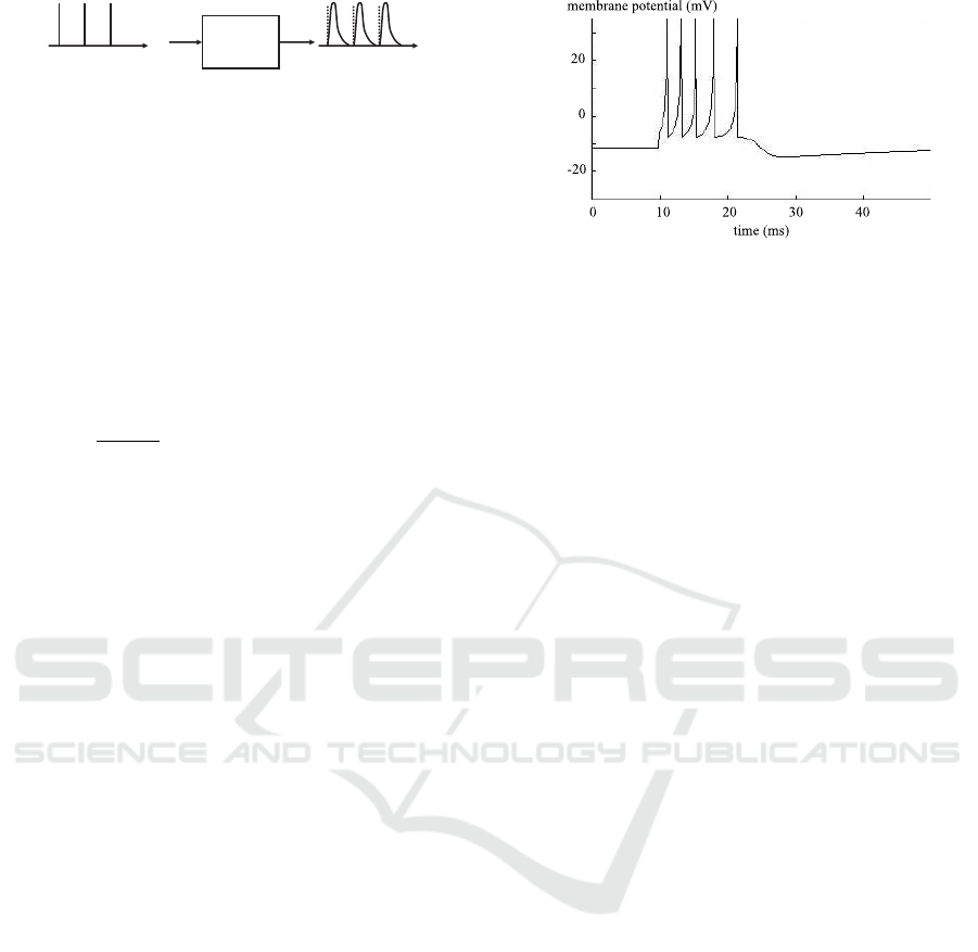
Figure 2: Model of the connections of i-th spiking neuron

in the SNN.

In this paper we consider recurrent spiking neural

networks (RSNNs) in which integrate-and-ﬁre type

spiking neurons shown in Fig.1 are fully connected

through synaptic weights w

i, j

and time delay elements

i, j

(s). Figure 2 shows a schematic diagram of the

connection of the ith spiking neuron in the RSNN.

We let here the number of neurons composed in the

RSNN be M. The elements g

i, j

(s) determine shape

of post synaptic potentials, so called spike-response

function as shown in Fig. 3, or delay due to the

spike transmission between spiking neurons. Synap-

tic weights w

i, j

are multiplied by the time delay ele-

ments (w

i, j

× g

i, j

(s)). The input stimulus e

(t) of the

i-th SN is generated by the weighted sum of each out-

put y

i, j

(t) of the element g

i, j

(s) and the external input

(t). The input u

i, j

(t) of g

i, j

(s) is connected with

NCTA 2019 - 11th International Conference on Neural Computation Theory and Applications

480

)(s

i,j

)(

Figure 3: Spikes and spike-response function.

the output of the j-th neuron σ

(t). The connection

topology of the entire RSNN is given by

(t) =

∑

j=1

i, j

(t) + v

(t), (7)

i, j

(t) = σ

(t). (8)

For the convenience of the derivation of the learning

algorithms, the elements g

i, j

(s) are expressed in the

state space form:

i, j

(t)

= A

i, j

(t) + b

i, j

(t) (9)

i, j

(t) = c

i, j

(t) (10)

i, j

(0) = x

i, j

, i, j = 1,··· ,M (11)

i, j

(s) = c

i, j

(sI − A

i, j

)

−1

i, j

where x

i, j

(t): N dimensional state vector, x

i, j

: N di-

mensional initial state vector and the dimensions of

the system matrices and vectors A

i, j

, b

i, j

and c

i, j

are

N × N, N × 1 and 1 × N, respectively. Equations

(1)∼(11) give the whole description of the RSNN

considered in this paper.

3 PROPOSED METHOD

3.1 Examples of Firing Patterns

In biological neural networks of living organisms,

various ﬁring patterns of nerve cells are observed.

The purpose of this paper is to propose a learning

method of neural network that produces such ﬁring

patterns. Here we introduce two examples of such ﬁr-

ing patterns observed in biological neural networks of

living organisms like human brains. One typical ex-

ample is a burst ﬁring pattern. It is a ﬁring pattern

as shown in Fig. 4, in which the number of ﬁrings

suddenly increases and decreases and the ﬁring time

interval and the non-ﬁring time interval are clearly di-

vided. In the ﬁgure an example of the time evolution

of the membrane potential of a neuron which gener-

ates burst ﬁring is shown. Another typical example is

a periodic ﬁring pattern. It is a ﬁring pattern in which

a same ﬁring pattern is repeated with a constant pe-

riod. In both ﬁring patterns, burst and periodic ﬁring

patterns, there could exist various ﬁring patterns de-

pending on ﬁring time, ﬁring frequency and so on.

Figure 4: An example of burst ﬁring.

3.2 Formulation of Learning Problems

3.2.1 Learning Problem for Generating Various

Firing Patterns

We now formulate the learning problem which real-

izes various ﬁring patterns. As stated above, in burst

ﬁring patterns the ﬁring time interval and the non-

ﬁring time interval are clearly divided. In order to

realize this, it is necessary to divide total time inter-

val into some sub time intervals and specify a desired

ﬁring pattern to each sub time interval.

Suppose that the RSNN operates starting at time

t = 0 and ﬁnishing at time t = t

and the total time

interval is 0 ≤ t < t

. For each neuron, say the i-th

SN denoted by SN

in the RSNN, we divide the total

time interval into sub time intervals and the number

of sub time intervals is denoted by S

. For the i-th SN,

let tv

-th sub time interval be t

i,tv

≤ t < t

i,tv

,(tv

1,2, ··· ,S

), where the start time t

i,tv

and the ﬁnish

time t

i,tv

satisfy the following equations.

i,tv

= t

i,tv

(i = 1,2,·· · , M;tv

= 1, ·· · , S

− 1)

i,1

= 0, t

i,S

= t

(i = 1,2,·· · , M) (12)

We now formulate the learning problem which re-

alizes various ﬁring patterns. We already pro-

posed a learning method of the RSNNs described by

(1)∼(11), in which the learning problem is formulated

such that the number of spikes emitted by SN and

their ﬁring instants coincide with given desired num-

bers of spikes and their desired ﬁring instants for the

interval [0,t

] (Selvaratnam and Mori, 2000; Kuroe

and Ueyama, 2010). In this paper, in order to real-

ize various ﬁring patterns, in addition to the learning

problem in (Selvaratnam and Mori, 2000; Kuroe and

Ueyama, 2010) we consider the learning problems in

which desired number of spikes without specifying

their ﬁring instant is given, and desired values of up-

per and/or lower limit of the number of spikes emitted

by SN are given. The learning problem is formulated

as follows.

Learning Method of Recurrent Spiking Neural Networks to Realize Various Firing Patterns using Particle Swarm Optimization

481

[Learning Problem]

Determine the values of the synaptic weights w

i, j

such

that the RSNN generates the desired spike sequence

if one of the values of the following items is speciﬁed

for any given neuron SN

in the RSNN and any given

sub time interval t

i,tv

≤t<t

i,tv

a) the number of spikes and their ﬁring instants,

b) the number of spikes,

c) the value of upper limit of the number of spikes,

d) the value of lower limit of the number of spikes or

e) the values of lower and upper limits of the number

of spikes.

Let the set of the neurons SN

which one of the items

a)–e) is speciﬁed be O and the set of the indexes

of the sub time intervals which one of the items

a)–e) is speciﬁed be U

. For the sub time interval

i,tv

≤t<t

i,tv

(tv

∈ U

), let the number of spikes which

emits be K

i,tv

, and the time instant of k

i,tv

-th

spike be t

i,k

i,t v

i,tv

= 1, 2,··· ,K

i,tv

). We introduce

the measures which represent discrepancies between

i,tv

, t

i,k

i,t v

and their speciﬁed values in a)–e) as cost

functions, denoted by J

i,tv

i,k

i,t v

i,tv

), and deﬁne

the total cost function as follows.

∑

i∈O

∑

∈U

i,tv

i,k

i,t v

i,tv

) (13)

where α

i,tv

are weight coefﬁcients. The def-

inition of J

i,tv

will be given in the next sec-

tion. Letting the learning parameters be X

1,1

1,2

,·· ·,w

i, j

,·· ·,w

M,M

), the learning problem

here is reduced to the following optimization prob-

lem:

Minimize J

(14)

w.r.t. X

3.2.2 Learning Problem for Generating Periodic

Firing Patterns

In order to make the network generate persistent pe-

riodic phenomena it should be a nonlinear dynamical

system like the RSNNs described by (1)∼(11). Here

we formulate the learning problem which generates

various patterns in the previous subsection and makes

them periodic with a given desired period T . In or-

der to make them periodic, the state variables p

and

i, j

(t) of the RSNN must satisfy the conditions:

(t) = p

(t + T ), x

i, j

(t) = x

i, j

(t + T ). (15)

The problem here is to determine the values of the

network parameters which minimize the cost func-

tion J

and make the conditions (15) being satisﬁed

simultaneously. We introduce another cost function

to realize the conditions. Note that the initial states

of the RSNN which realize the conditions (15) are

unknown. As the learning parameters we choose

not only the synaptic weights w

i, j

but also the initial

states of the RSNN, p

and x

0,n

i, j

(i = 1,2,·· · , M; n =

1,2, ··· ,N). Deﬁning X

= (w

1,1

,·· ·,w

i, j

,·· ·,w

M,M

,·· ·,p

, x

0,1

1,1

,·· ·,x

0,n

i, j

,·· ·,x

0,N

M,M

), the learning

problem here is reduced to the following optimization

problem:

Minimize J

+ βJ

(16)

w.r.t. X

subject to |p

| < s

is the cost function realizing the periodicity condi-

tion (15), the deﬁnition of which is given in the next

section, and β is a weight coefﬁcient. Note that the

constraint |p

| < s

is set to prevent the fact that SN

always ﬁres at the initial time t = 0 if |p

| ≥ s

3.3 Deﬁning the Cost Functions

It is known that, since PSO is an optimization method

that uses only values of a cost function and does not

require its continuity or the existence of its gradient,

various cost functions can be set according to opti-

mization problems. It is, therefore, important what

kind of cost functions are set. We now propose cost

functions which realize the items a)–e) and the peri-

odicity condition (15).

3.3.1 Cost Function for Firing Instants

Let the desired number of spikes emitted by SN

for

the time interval t

i,tv

≤t<t

i,tv

be K

i,tv

and their de-

sired ﬁring instants be t

i,k

i,t v

i,tv

=1,2,· ·· ,K

i,tv

). In

order to realize that the number of spikes emitted by

each SN

and their ﬁring instants coincide with the

given desired ones, we deﬁne the following cost func-

tion J

i,t v

∑

i,t v

i,k

i,t v

−t

i,k

i,t v

+ J

111

(17)

where

111











i,t v

∑

i,t v

i,k

i,t v

−t

i,k

i,t v

,(K

i,tv

> K

i,tv

)

i,t v

∑

i,t v

i,k

i,t v

−t

i,K

i,t v

,(K

i,tv

< K

i,tv

)

0, (K

i,tv

= K

i,tv

)

NCTA 2019 - 11th International Conference on Neural Computation Theory and Applications

482

and ex is the exponentiation parameter which is usu-

ally chosen as ex = 1 or 2. J

111

is a penalty func-

tion which is applied when the number of spikes

emitted by SN

does not coincident with the de-

sired one. When K

i,tv

> K

i,tv

, in order to avoid the

excess number of spikes being ﬁred we set provi-

sional teaching signals for the excess spikes. Let

i,k

i,t v

be the timings of the provisional teaching

signals to the ﬁring instants of the excess spikes

i,k

i,t v

i,tv

= K

i,tv

+ 1,·· · , K

i,tv

. We choose values

of t

i,k

i,t v

to be larger enough than t

i,k

i,t v

>> t

When K

i,tv

< K

i,tv

, in order to make each SN

gen-

erate additional spikes we set the penalty as follows.

Considering that at the ﬁring instant t

i,K

i,t v

of the last

actual spike emitted by SN

the missing K

i,tv

− K

i,tv

number of spikes ﬁre simultaneously, we set the error

between the last actual ﬁring instant and the desired

ﬁring instants as in the second case of J

111

3.3.2 Cost Function for the Upper and Lower

Limits of the Number of Spikes

Let the desired upper and lower limit values of the

number of spikes emitted by SN

for the time inter-

val t

i,tv

≤t<t

i,tv

be K

i,tv

and K

i,tv

, respectively. The

cost function for the upper limit is set so that its value

increases as the number of spikes emitted by SN

ex-

ceeds the upper limit value K

i,tv

as follows.

= max(K

i,tv

− K

i,tv

,0)

(18)

The cost function for the lower limit is set so that its

value increases as the number of spikes emitted by

lowers the lower limit value K

i,tv

as follows.

= max(K

i,tv

− K

i,tv

,0)

(19)

3.3.3 Cost Function for Generating Periodic

Firing Patterns

In order to make ﬁring pattern be periodic with period

T , the state variables p

(t) and x

i, j

(t) of the RSNN

must satisfy the conditions (15). The cost function J

for the problem (16) is set so as to realize the condi-

tions (15) as follows.

∑

i=1



− p

T )|

∑

j=1

∑

n=1

0,n

i, j

− x

i, j

T )|



(20)

It is theoretically enough to let N

= 1, however, we

introduce the parameter N

for numerical accuracy.

The items a)–e) in Subsection 3.2.1 can be real-

ized by appropriately choosing from the cost func-

tions J

, J

deﬁned in the above section and

combining them as follows.

a) J

b) J

+ J

(Let K

= K

c) J

d) J

e) J

+ J

3.4 Learning Method based on the PSO

The cost function J

deﬁned by (17) is differen-

tiable with respect to the network parameters X

1,1

1,2

,·· ·,w

i, j

,·· ·,w

M,M

) if ex = 2, and gradient

based learning methods were proposed in (Selvarat-

nam and Mori, 2000; Kuroe and Ueyama, 2010) for

RSNNs. Since the other cost functions are not dif-

ferentiable, we use the particle swarm optimization

method (PSO) (Kennedy and Eberhart, 2001) in order

to solve the optimization problems (14) and (16). In

the following we explain the outline of the PSO.

Consider an optimization problem of determining

values of N

decision variables X = (x

,·· ·,x

)

which minimize a cost function J(X). In the PSO, a

swarm is prepared and its all member particles are

used for solving the problem. Let P be the num-

ber of the particles (the swarm size), and X

p,k

,·· ·,x

p,k

,·· ·,x

p,k

) be the candidate solution of p-

th particle (p = 1, 2,· ·· ,P) at the k-th iteration. The

candidate solution of p-th particle at the next ((k +1)-

th) iteration is determined based on the update equa-

tion of the PSO as follows.

p,k+1

= x

p,k

+ 4x

p,k+1

(21)

where

p,k+1

= W 4x

p,k

+ C

rand

()

p,k

(pbest

p,k

− x

p,k

)

+ C

rand

()

p,k

(gbest

− x

p,k

) (22)

and the update value 4X

= (4x

,·· ·,4x

,·· ·,

) is called the velocity vector of the p-th parti-

cle, rand

()

p,k

,rand

()

p,k

are uniform random num-

bers in the range from 0 to 1, W is a weight pa-

rameter called the inertia weight, and C

and C

are

weight parameters called the acceleration coefﬁcients.

pbest

p,k

= (pbest

p,k

, ··· ,pbest

p,k

, ··· ,pbest

p,k

)) is

called the personal best which is the best candidate

solution found by the p-th particle until the k-th it-

eration and gbest

=(gbest

,·· · ,gbest

) is

called the global best which is the best candidate so-

lution found by all the members of the swarm, and

they are given as: pbest

p,k

= x

p,k

∗

and gbest

pbest

∗

where k

∗

= argmin

1≤k

≤k

J(X

p,k

) and p

∗

argmin

1≤p≤P

J(pbest

p,k

Learning Method of Recurrent Spiking Neural Networks to Realize Various Firing Patterns using Particle Swarm Optimization

483

4 NUMERICAL EXPERIMENTS

4.1 Problems and Experiment

We prepare the following three learning problems for

experiments and apply the proposed method to them.

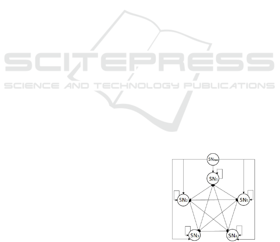
Experiment 1

We consider the RSNN consists of fully connected

ﬁve neurons SN

(i = 1, 2,. ..,5) and one input neu-

ron SN

input

which generates a triggering input v

(t)

as shown in Fig. 5. We let the triggering input be

(t) = δ(0). In this problem the total time inter-

val [0.0,5.0) is divided into two sub time intervals

[0.0,2.5) and [2.5,5.0). The desired ﬁring sequences

shown in Table 1 are given to the RSNN, where it is

trained so as that SN

ﬁres the desired numbers of

spikes for each sub time interval and without assign-

ing their ﬁring instants, and SN

, SN

and SN

ﬁre the

desired lower and/or upper limit values of the number

of spikes. SN

is not given desired ﬁring sequences.

This experiment is a learning problem in which the

items b), c), d) and e) in 3.2.1 is speciﬁed.

Experiment 2

Experiment 2 is a learning problem in which the item

b) in 3.2.1 is speciﬁed and burst ﬁrings with the de-

sired number of spikes are realized. We consider the

same RSNN as in Experiments 1 shown in Fig. 5.

The time interval [0.0,5.0) is divided into three sub

time intervals [0.0,1.0), [1.0,1.5) and [1.5, 5.0). The

desired ﬁring sequences shown in Table 2 are given to

of the RSNN so that it emits a speciﬁed desired

number of spikes for the time interval [1.0,1.5) and it

does not ﬁre for the other time intervals [0.0,1.0) and

[1.5,5.0). The experiments are carried out for two

conditions I ( K

1,2

= 10) and II ( K

1,2

= 20).

Experiment 3

Experiment 4 is a learning problem in which the

item b) in 3.2.1 is speciﬁed and a periodic ﬁring

is realized. We consider the RSNN consists of

two neurons SN

(i = 1,2) which are mutually con-

nected as shown in Fig. 6 because neural oscilla-

tors are usually realized by using such fully con-

nected two neuron networks. The total time interval

is [0.0,20.0) and it is divided into ﬁve sub time inter-

vals [0.0, 4.0),[4.0, 8.0),[8.0, 12.0),[12.0, 16.0) and

[16.0,20.0). The desired ﬁring sequences shown in

Table 3 are given to SN

of the RSNN so that it ﬁres a

speciﬁed desired number of spikes for each sub time

interval. In addition to that the periodic conditions

(15) are given so that the RSNN generates a periodic

ﬁring pattern with the period T = 20.

In order to solve the problems of the above

experiments it is necessary to choose appropriate

cost functions in the optimization problems (14) and

(16). We choose the following cost functions for each

problem:

Ex. 1: J =

∑

i∈O

∑

∈U

+ J

)

Ex. 2-I, II: J =

∑

i∈O

∑

∈U

+ J

)

Ex. 3: J =

∑

i∈O

∑

∈U

+ J

) + J

In the experiments the parameters of the RSNN

are set as follows. For all experiments we choose

= 0.2, s

= 1.0 and the parameters in the state space

model of the elements g

i, j

(s) are: N = 2 and A

i, j



−3.0 0.0

0.0 −6.0



, b

i, j



1.0



, c

i, j

= (1.0,−1.0). In

Experiment 1 and 2 the initial states are chosen as

= 0.0, x

i, j



0.0



For all the experiments the exponentiation param-

eter ex of the cost functions is chosen as ex = 2. For

Experiment 3 the parameter N

of the cost function

is chosen as N

= 1 and the weight coefﬁcient γ is

chosen as γ = 25.

For all experiments the parameters of the parti-

cle swarm optimization are chosen as follows. The

parameters of the update equations (21) and (22)

(W,C

) are chosen:(W,C

) = (0.7,1.4,1.4),

the number of the particles is P = 100 or P = 200,

the maximum number T

max

of learning iterations is

max

= 5000. In each experiment the learning itera-

tion ﬁnishes when the number of the learning iteration

reaches T

max

. For each particle the initial values of the

candidate solution and its velocity, w

p,0

i, j

and 4w

p,0

i, j

are determined randomly within the range [−10,10].

In Experiment 3 for each particle the initial values of

the candidate solution and its velocity, p

, 4p

, x

0,n

i, j

and 4x

0,n

i, j

are determined randomly within the range

[−1,1] by considering the fact that s

= 1.0.

Figure 5: Fully connected ﬁve neurons SN

(i = 1,... , 5) and

one input neuron SN

input

NCTA 2019 - 11th International Conference on Neural Computation Theory and Applications

484

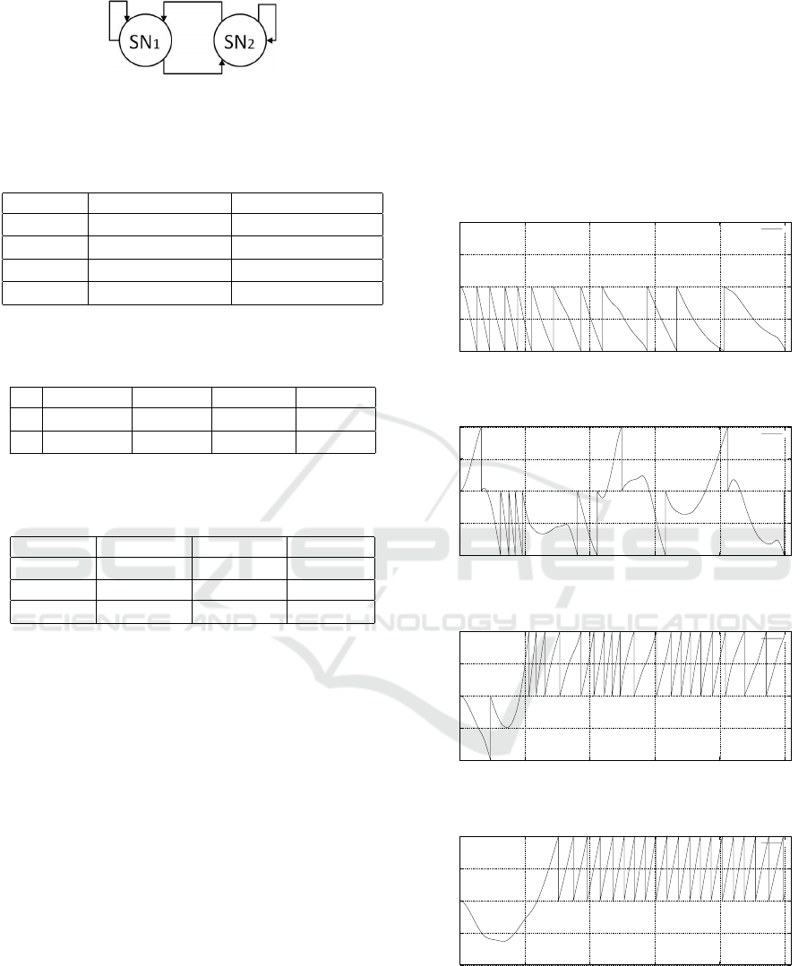
Figure 6: RSNN consists of mutually connected two neu-

rons SN

(i = 1, 2).

Table 1: Desired Firing Sequences (Ex. 1).

Ex. 1 (S

= 2,t

= 5.0)

i,tv

) [0.0,2.5) [2.5,5.0)

1,1

= 8 K

1,2

= 3

2,1

= 8 K

2,2

= 3

3,1

= 10 K

3,2

= 10

4,1

= 10,K

4,1

= 5 K

4,2

= 20,K

4,2

= 15

Table 2: Desired Firing Sequences (Ex. 2).

Ex. 2 (S

= 3,S

,·· ·,S

= 1,t

= 5.0)

i,tv

, t

i,tv

) [0.0,1.0) [1.0,1.5) [1.5,5.0)

I SN

1,1

= 0 K

1,2

= 10 K

1,3

= 0

II SN

1,1

= 0 K

1,2

= 20 K

1,3

= 0

Table 3: Desired Periodic Firing Sequences (Ex. 3).

Ex. 3 (S

= 5,t

= 20.0)

i,tv

) [0.0,4.0) [4.0,8.0) [8.0,12.0)

1,1

= 4 K

1,2

= 4 K

1,3

= 4

i,tv

) [12.0,16.0) [16.0,20.0)

1,4

= 4 K

1,5

= 4

4.2 Results and Discussions

We applied the proposed learning method to each ex-

periment. The results are shown here.

Result of Experiment 1

After training the RSNN shown in Fig. 5 by the pro-

posed method we run it by the same triggering signal

(t) = δ(0) from the input neuron SN

input

and ob-

serve its behavior. Figures 7, 8, 9 and 10 show ex-

amples of time evolutions of the internal state p

(t)

of SN

, p

(t) of SN

, p

(t) of SN

and p

(t) of SN

obtained from the result, respectively. It is observed

from the ﬁgures that SN

, SN

and SN

emit

the desired ﬁring sequences shown in Table 1, which

implies that the learning is successfully done by the

proposed method.

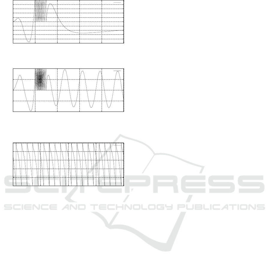
Result of Experiment 2

Figures 11 and 12 show examples of time evolutions

of the internal state p

(t) of SN

obtained from the

results Ex. 3-I and Ex. 3-II, respectively. It is ob-

served from the ﬁgures the burst ﬁrings with the de-

sired number of spikes are realized and the learning is

successfully done by the proposed method.

Result of Experiment 3

After training the RSNN shown in Fig. 6 by the pro-

posed method, we run it with the obtained initial con-

dition and observe its behavior. Note that the RSNN

shown in Fig. 6 has no input neuron and it is triggered

by the initial conditions. Figures 13 shows an exam-

ple of the time evolution of the internal state p

(t) of

obtained from the result. It is observed that the

periodic ﬁrings with the desired number of spikes are

realized.

-1

-0.5

0.5

0 1 2 3 4 5

(t)

time

Figure 7: Time evolution of p

(t) after learning in Ex. 1.

-1

-0.5

0.5

0 1 2 3 4 5

(t)

time

Figure 8: Time evolution of p

(t) after learning in Ex. 1.

-1

-0.5

0.5

0 1 2 3 4 5

(t)

time

Figure 9: Time evolution of p

(t) after learning in Ex. 1.

-1

-0.5

0.5

0 1 2 3 4 5

(t)

time

Figure 10: Time evolution of p

(t) after learning in Ex. 1.

Learning Method of Recurrent Spiking Neural Networks to Realize Various Firing Patterns using Particle Swarm Optimization

485

-1

-0.8

-0.6

-0.4

-0.2

0.2

0.4

0.6

0.8

0 1 2 3 4 5

(t)

time

Figure 11: Time evolution of p

(t) after learning in Ex. 2-I.

-1

-0.5

0.5

0 1 2 3 4 5

(t)

time

Figure 12: Time evolution of p

(t) after learning in Ex. 2-

II.

-1

-0.8

-0.6

-0.4

-0.2

0 5 10 15 20

(t)

time

Figure 13: Time evolution of p

(t) after learning in Ex. 3.

5 CONCLUSIONS

In biological neural networks of living organisms,

various ﬁring patterns of nerve cells have been ob-

served, typical example of which are burst ﬁrings and

periodic ﬁrings. The RSNNs are expected to realize

various complicated ﬁring patterns because of their

behavior as nonlinear dynamical systems. In this pa-

per we proposed a learning method which can real-

ize various ﬁring patterns for RSNNs. We consid-

ered several desired properties of a target RSNN and

proposed cost functions for realizing them. Since the

proposed cost functions are not differentiable with re-

spect to the learning parameters and their gradients

do not exist, we propose larning methods based on

the particle swarm optimization (PSO). Some exper-

imental examples were provided to show the validity

of the proposed method.

This work was ﬁnancially supported in part by

the Kansai University Fund for the Promotion and

Enhancement of Education and Research, 2018 and

JSPS KAKENHI (18K11483).

REFERENCES

Bohte, S. M., K., N., J., and Poutre, H. L. (2002). Error-

backpropagation in temporally encoded networks of

spiking neurons. Neurocomputing, Vol.48(Issues 1-

4):pp.17–37.

Gerstner, W., R. R. and van Hemmen, J. L. (1993a).

Why spikes? hebbian learning and retrieval of time-

resolved excitation patterns. Biological. Cybernetics,

Vol.69:pp.503–515.

Gerstner, W. and van Hemmen, J. L. (1993b). How to de-

scribe neural activities: Spikes, rates or assemblies?

Advances in Neural Information Processing Systems,

San Mateo, Vol.6:pp.363–374.

Izhikevich, E. (2007). Dynamical systems in Neuroscience

-The Geometry of Excitability and Bursting. MIT

Press.

Izhikevich, E. M. (2004). Which model to use for cortical

spiking neurons? IEEE Transactions on Neural Net-

works, Vol.15(No.5):pp.1063–1070.

Kennedy, J. and Eberhart, R. (2001). Swarm Intelligence.

Morgan Kaufmann Publishers.

Kuroe, Y. (1992). Learning method of recurrent neu-

ral networks. ISCIE Control and Information,

Vol.36(No.10):pp.634–643.

Kuroe, Y. and Ueyama, T. (2010). Learning methods

of recurrent spiking neural networks based on ad-

joint equations approach. Proc. of WCCI 2010 IEEE

World Congress on Computational Intelligence, pages

pp.2561–2568.

Lee, J.H., D. T. and Pfeiffer, M. (2016). Training deep spik-

ing neural networks using backpropagation. Frontiers

in Neuroscience, Vol.10(Article 508):pp.1–13.

Mass, W. (1996). On the Computational Complexity of Net-

work of Spiking Neurons, volume Vol.7. MIT Press.

Mass, W. (1997a). Fast sigmoidal networks via spiking neu-

rons. Neural Computation, Vol.9:pp.279–304.

Mass, W. (1997b). Networks of spiking neurons: The third

generation of neural network models. Neural Net-

works, Vol.10(No.9):pp.1659–1671.

Mass, W. and Bishop C., E. (1998). Pulsed Neural Nets.

MIT Press.

Rumelhart, D. E. and McClelland, J. L. (1986). Parallel

Distributed Processing, volume Vols. 1 and 2. MIT

Press.

Selvaratnam, K., K. Y. and Mori, T. (2000). Learning

methods of recurrent spiking neural networks - tran-

sient and oscillatory spike trains. Trans. of the Insti-

tute of Systems, Control and Information Engineers,

Vol.44(No.3):pp.95–104.

NCTA 2019 - 11th International Conference on Neural Computation Theory and Applications

486