Stochastic Information Granules Extraction for Graph Embedding and

Classiﬁcation

Luca Baldini

, Alessio Martino

and Antonello Rizzi

Department of Information Engineering, Electronics and Telecommunications, University of Rome "La Sapienza",

Via Eudossiana 18, 00184 Rome, Italy

Keywords:

Pattern Recognition, Supervised Learning, Granular Computing, Graph Embedding, Inexact Graph Matching.

Abstract:

Graphs are data structures able to efﬁciently describe real-world systems and, as such, have been extensively

used in recent years by many branches of science, including machine learning engineering. However, the

design of efﬁcient graph-based pattern recognition systems is bottlenecked by the intrinsic problem of how

to properly match two graphs. In this paper, we investigate a granular computing approach for the design

of a general purpose graph-based classiﬁcation system. The overall framework relies on the extraction of

meaningful pivotal substructures on the top of which an embedding space can be build and in which the

classiﬁcation can be performed without limitations. Due to its importance, we address whether information

can be preserved by performing stochastic extraction on the training data instead of performing an exhaustive

extraction procedure which is likely to be unfeasible for large datasets. Tests on benchmark datasets show that

stochastic extraction can lead to a meaningful set of pivotal substructures with a much lower memory footprint

and overall computational burden, making the proposed strategies suitable also for dealing with big datasets.

1 INTRODUCTION

Graphs are powerful data structures able to capture

relationships between elements. This representative

power in describing patterns under a structural and

topological viewpoint makes graphs a ﬂexible and ac-

curate abstraction especially when nodes and/or edges

can be equipped with labels (in this case, we refer to

as labelled graphs). Indeed, they have been widely

used to model a plethora of real-world phenomena,

including biological systems (Giuliani et al., 2014;

Krishnan et al., 2008; Di Paola and Giuliani, 2017),

functional magnetic resonance imaging (Richiardi

et al., 2013), computer vision (Bai, 2012) and online

handwriting (Del Vescovo and Rizzi, 2007b). On the

other hand, it is rather common in pattern recognition

to represent the input pattern as a feature vector ly-

ing in an n-dimensional vector space. This is mainly

due to the relatively simple underlying math whether

some properties are satisﬁed. In fact, the resulting

space can easily be equipped by an adequate metric

satisfying the properties of non-negativity, identity,

symmetry and triangle inequality (P˛ekalska and Duin,

https://orcid.org/0000-0003-4391-2598

https://orcid.org/0000-0003-1730-5436

https://orcid.org/0000-0001-8244-0015

2005; Martino et al., 2018a; Weinshall et al., 1999).

This can not be easily achieved in structured domains

and, for this reason, the main drawback when repre-

senting entities with graphs is the unpractical, non-

geometric space to whom they belong to. A rather

natural approach to tackle this problem when design-

ing a classiﬁcation system, is to use an ad-hoc dissim-

ilarity measure working directly in the input space:

this allows to reuse some of the well-known pattern

recognition techniques for supervised learning, e.g.

the K-Nearest Neighbour (K-NN) algorithm (Cover

and Hart, 1967). Related to this approach, we con-

sidered Graph Edit Distances (GEDs) (Neuhaus and

Bunke, 2007) that operate directly in the structured

domain (i.e., graphs), measuring the dissimilarity be-

tween two graphs, say G

and G

, as the minimum

cost sequence of atomic operations (namely, substi-

tution, deletion and insertion of nodes and/or edges)

needed to transform G

into G

. A very interest-

ing strategy that has gained much attention relies on

Graph Kernels (Vishwanathan et al., 2010; Ghosh

et al., 2018): these methods exploit the so-called ker-

nel trick, that is the inner product between graphs in a

vector space induced by a (semi)deﬁnite positive ker-

nel function. The classiﬁcation task can heavily rely

on well-known kernelized algorithms, the seminal ex-

Baldini, L., Martino, A. and Rizzi, A.

Stochastic Information Granules Extraction for Graph Embedding and Classiﬁcation.

DOI: 10.5220/0008149403910402

In Proceedings of the 11th International Joint Conference on Computational Intelligence (IJCCI 2019), pages 391-402

ISBN: 978-989-758-384-1

391

ample being Support Vector Machines (Cortes and

Vapnik, 1995). The last method, that is closely related

to this work, is Graph Embedding. In this approach,

the input pattern from the structured graphs domain

G is mapped into an embedding space D. Clearly, the

designing of the mapping function φ : G → D with

D ⊆ R

is crucial in this procedure and some effort

must be ensured to ﬁll the informative and seman-

tic gap between the two domains. For this purpose,

a Granular Computing (Bargiela and Pedrycz, 2008)

approach based on the extraction of information gran-

ules together with symbolic histograms (Del Vescovo

and Rizzi, 2007a) can be pursued in order to obtain

an efﬁcient mapping function able to reﬂect the infor-

mation carried by the structured data into the vector

space. This method allows the use of common classi-

ﬁcation and data-driven systems and can achieve not

only performance similar to the state-of-art classiﬁers

(Bianchi et al., 2014a), but can also provide useful in-

formation through the extracted granules, as they are

human-interpretable. Unfortunately, an heavy com-

putational effort is necessary and often, as the dataset

size increases, the problem may become unfeasible,

especially under the memory footprint viewpoint.

In this paper, starting from the classiﬁcation sys-

tem developed by (Bianchi et al., 2014a), we explore

an alternative approach for substructures extraction

that will be used to synthesize the alphabet, i.e. the set

of information granules on the top of which the em-

bedding space is built. In particular, a lighter stochas-

tic procedure has been developed and compared to

exhaustive method from (Bianchi et al., 2014a); this

procedure takes advantage of Breadth First Search

(BFS) and Depth First Search (DFS) algorithms for

graph traversing.

This paper is organized as follows: in Section 2

we give an overview of Granular Computing both as

an information processing paradigm and as a frame-

work in order to build data-driven classiﬁcation sys-

tems for structured data; in Section 3 we introduce

GRALG, the graph-based classiﬁcation system core

of this work, highlighting the improvements with re-

spect to its original implementation. Section 4 regards

computational results both in terms of performances

and computational burden with respect to the origi-

nal implementation and, ﬁnally, Section 5 draws some

conclusions and future directions.

2 EMBEDDING VIA DATA

GRANULATION

Granular Computing is often described as a human-

centered information processing paradigm (Howard

and Lieberman, 2014; Yao, 2016) based on formal

mathematical entities known as information gran-

ules (Han and Lin, 2010; Bargiela and Pedrycz,

2006). The human-centered computational concept

in soft computing and computational intelligence was

initially developed by Lofti Zadeh through fuzzy

sets (Zadeh, 1979) that exploits human-inspired ap-

proaches to deal with uncertainties and complexities

in data. The process of ’granulation’, intended as the

extraction of meaningful aggregated data, mimics the

human mechanism needed to organize complex data

from the surrounding environment in order to sup-

port decision making activities and describe the world

around (Pedrycz, 2016). For this reason, Granular

Computing can be deﬁned as a framework for analyz-

ing data in complex systems aiming to provide human

interpretable results (Livi and Sadeghian, 2016).

The importance of information granules resides in

the ability to underline properties and relationships

between data aggregates. Speciﬁcally, their synthe-

sis can be achieved by following the indistinguisha-

bility rule, according to which elements that show

enough similarity, proximity or functionality shall be

grouped together (Zadeh, 1997). With this approach,

each granule is able to show homogenous semantic in-

formation from the problem at hand (Pedrycz, 2010).

Furthermore, data at hand can be represented using

different levels of ’granularity’ and thus different pe-

culiarities of the considered system can emerge (Yao,

2008; Pedrycz and Homenda, 2013; Yao and Zhao,

2012; Wang et al., 2017; Yang et al., 2018). When

analyzing a system with high level of detail, one shall

expect a huge number of very compact information

granules since, straightforwardly, ﬁner details are of

interest. On the other hand, the level of abstraction

increases when decreasing the granularity level: as a

result, one shall expect a lower number of very pop-

ulated, yet less compact, information granules. De-

pending on this resolution, a problem may exhibit dif-

ferent properties and different atomic units that show

different representations of the system as a whole.

Clearly, an efﬁcient and automatic procedure to se-

lect the most suitable level of abstraction according to

both the problem at hand and the data description is

of utmost importance.

A mainstream approach in order to synthesize a

possibly meaningful set of information granules can

be found in data clustering. Since its direct connec-

tion with the concept of ’granules-as-groups’, cluster

analysis has been widely explored in the context of

granular computing (Pedrycz, 2005; Pedrycz, 2013).

When designing a clustering method for information

granules synthesis, the parameters of the algorithm

must be tuned in an appropriate way in order to select

NCTA 2019 - 11th International Conference on Neural Computation Theory and Applications

392

the relevant features at a suitable resolution (granu-

larity) for the problem at hand. According to (Ding

et al., 2015), typically three main factors can impact

the resulting data partitioning: (dis)similarity mea-

sure, threshold parameter and cluster representatives.

The threshold deﬁnes whether a given pattern belongs

or not to a speciﬁc cluster. In our point of view,

this threshold changes the granularity and therefore

the level of detail considered. A typical clustering

algorithm that endows a threshold in order to deter-

mine pattern-to-cluster assignments is the Basic Se-

quential Algorithmic Scheme (BSAS) (Theodoridis

and Koutroumbas, 2008) that performs a so-called

free clustering procedure, i.e. the number of clusters

shall not be deﬁned a-priori as in other data clustering

paradigms, notably k-clustering (Martino et al., 2017;

Martino et al., 2018b; Martino et al., 2019). Varying

the threshold parameter impacts on how patterns will

be aggregated into clusters. A suitable (dis)similarity

function is in charge to measure the (dis)similarity

in order to aggregate data entities in a proper man-

ner. Since the clustering procedure is usually per-

formed in the input (structured) domain, not only the

(dis)similarity measure, but also the cluster represen-

tative shall be tailored accordingly. In order to repre-

sent clusters in structured domains, the medoid (also

called MinSOD) is usually employed (Del Vescovo

et al., 2014) mainly due to the following reason: its

evaluation relies only on pairwise dissimilarities be-

tween patterns belonging to the cluster itself, with-

out any algebraic structures that can not be deﬁned

in non-geometric spaces (Martino et al., 2017). The

clusters representatives from the outcoming partition

can be considered as symbols belonging to an alpha-

bet A = {s

,...,s

}: these symbols are the pivotal

granules on the top of which the embedding space can

be built thanks to the symbolic histograms paradigm.

According to the latter, each pattern can be described

as an m-length integer-valued vector which counts in

position i the number of occurrences of the i

symbol

drawn from the alphabet. The embedding space can

ﬁnally be equipped with algebraic structures such as

the Euclidean distance or the dot product and standard

classiﬁcation systems can be used without limitations.

3 THE GRALG CLASSIFICATION

SYSTEM

GRALG (GRanular computing Approach for La-

belled Graphs) is a general purpose classiﬁcation sys-

tem suitable for dealing with graphs and based on

Granular Computing. GRALG has been originally

proposed in (Bianchi et al., 2014a) and lately suc-

cessfully applied in the context of image classiﬁca-

tion (Bianchi et al., 2014b; Bianchi et al., 2016). In

this Section, the main blocks of the system are de-

scribed separately (Sections 3.1–3.4), along with the

way they cooperate in order to perform the training

(Section 3.5) and testing phases (Section 3.6).

3.1 Extractor

The goal of this block regards the extraction of sub-

structures from the input set S ⊂ G. In the origi-

nal GRALG implementation, this procedure used to

compute exhaustively the set of possible subgraphs

from any given graph G ∈ S. The maximum order o,

namely the maximum number of vertices for all sub-

graphs, is an input parameter which must be deﬁned

by the end-user. Obviously, the complexity of the pro-

cedure strongly depends on this parameter: in fact,

the asymptotically combinatorial behaviour of an ex-

haustive extraction makes this method unfeasible for

large graphs and/or for high value of o, both in terms

of running time and memory usage. The procedure

used to expand each node of a given graph to a pos-

sible subgraph of order 2, caching in memory the re-

sulting substructures, and then expanding and storing

them iteratively until the desired maximum order o is

reached. At the end of the extraction procedure, the

resulting set of substructures S

is returned.

3.1.1 Random Subgraphs Extractor based on

BFS and DFS

The new procedure randomly draws a graph G ∈ S

and then selects a seed node v ∈ G for a traversal strat-

egy based on either BFS or DFS in order to extract a

subgraph. Both the extractions (graph G from S and

node v from G) are performed with uniformly random

distribution. Alongside o (maximum subgraph order),

a new parameter W determines the cardinality of S

Algorithm 1: Random Extractor.

procedure EXTRACTRND(Graph Set

S = {G

,.. .,G

} with G = {V ,E}, W max

size of subgraphs set, empty set of subgraphs S

, o

max order of extracted subgraph)

while |S

| ≤ W do

for order = 1 to o do

Random extract a graph G from S

Random extract a vertex v from V

g = EXTRACT(G,v,order)

= S

∪ g

return Subgraph Set S

with |S| = W

Stochastic Information Granules Extraction for Graph Embedding and Classiﬁcation

393

Algorithm 1, which summarizes this procedure, relies

on a procedure called EXTRACT (separately described

in Algorithm 2) that performs a graph traverse using

one of the two well-known algorithms:

Breadth First Search: Starting from a node v, BFS

performs a traverse throughout the graph explor-

ing ﬁrst the adjacent nodes of v, namely those with

unitary distance, and then moving farther only af-

ter the neighbourhood is totally discovered. A

First-In-First-Out policy is in charge to organize

the list of neighbours for the considered vertex, in

order to give priority to adjacent nodes. The algo-

rithm can be summerized as follow:

1. Select the starting vertex v.

2. Push v in a queue list Q.

3. Pop u the ﬁrst element of the queue from Q.

4. For each neighbour s of u, push s to Q if s is not

mark as visited.

5. Mark u as a visited vertex.

6. Repeat 3-5 until Q is empty.

Depth First Search: In this strategy, a given graph

is traversed starting from a seed vertex v, but un-

like the BFS search, the visit follows a path with

increasingly distance from v and backtracks only

after all the vertices from the selected path are dis-

covered. A Last-In-First-Out policy is in charge to

organize the list of neighbours for the considered

vertex, in order to visit in-depth vertices ﬁrst. The

steps of the algorithm are:

1. Select the starting vertex v.

2. Push v in a stack list S.

3. Pop u the last element from stack S.

4. For each neighbour s of u, push s in S if s is not

marked as visited.

5. Mark u as visited.

6. Repeat 3-5 until S is empty.

Algorithm 2: BFS/DFS graph extraction.

procedure EXTRACT(Graph G, Vertex v, order ac-

tual order of extracted subgraph)

graph g of vertex V

and E

initially empties

repeat

} ← BFS/DFSsearch with seed

node v

until |V

| = order

g = {V

}

return g

In Algorithm 2, these methods are employed to pop-

ulate the set of vertices V

and edges E

for the sub-

graph g: a vertex is added to V

as soon as it is marked

as visited, whereas an edge is added to E

by consid-

ering the current and the last visited vertices.

3.2 Granulator

This module is in charge to compute the alphabet

symbols A starting from the subgraphs belonging to

the set S

, as returned by the Extractor deﬁned in Al-

gorithm 1. The information granules are synthesized

by performing the BSAS clustering algorithm on S

The BSAS algorithm relies on two parameters Q and

θ, respectively the maximum number of allowed clus-

ters and a threshold dissimilarity below which a pat-

tern can be included in its nearest cluster

. Regarding

θ, it is worth noting that different values lead to dif-

ferent partitions and a binary search is deployed to

generate an ensemble of partitions, each of which is

obtained with a different value for θ. For every clus-

ter C in the resulting partitions, a cluster quality index

F(C) is deﬁned as:

F(C) = η · Φ(C) +(1 − η) ·Θ(C) (1)

where the two terms Φ(C) and Θ(C) are deﬁned re-

spectively as:

Φ(C) =

|C| − 1

∑

d(g

∗

) (2)

Θ(C) = 1 −

|C|

(3)

where, in turn, g

∗

is the representative of cluster C

and g

the i

pattern in the cluster. In other words,

the quality index (1) sees a convex linear combination

between the compactness Φ(C) and the cardinality

Θ(C), weighted by a parameter η ∈ [0,1]. From Sec-

tion 2, g

∗

is the MinSOD of cluster C, deﬁned as the

element that minimizes the sum of pairwise distances

with respect to all other patterns in the cluster. The

dissimilarity measure driving both Eq. (2) and the

overall clustering procedure is deﬁned as a weighted

GED, described in details in Section 3.2.1. Eq. (1)

needs to be evaluated for all clusters in the partitions

(regardless of the corresponding θ), yet only repre-

sentatives belonging to clusters whose quality index

is above a threshold τ

are eligible to be included in

A: in this way, only well-formed clusters (i.e., com-

pact and populated) are considered.

3.2.1 Dissimilarity Measure and Inexact Graph

Matching

The core dissimilarity measure in GRALG is a

weighted GED, which is based on the same ratio-

If a pattern cannot be included in one of the available clus-

ters, it can be used to initialize a new cluster, provided that

the number of already-available clusters is below Q.

NCTA 2019 - 11th International Conference on Neural Computation Theory and Applications

394

nale behind other well-known edit distances, such as

the Levenshtein distance between strings (Cinti et al.,

2019). Accordingly, it is possible to deﬁne some edit

operations on graphs: deletion, insertion, substitution

of both nodes and edges. Each of these operations

can be possibly associated to a weight in order to tune

the penalty induced by a particular transformation.

In GRALG, six weights for edit operations are taken

into account in order to establish the importance of

substitutions, deletions and insertions for vertices and

edges.

Formally speaking, the GED between G

and G

can be deﬁned as a function d : G ×G → R, such that:

d(G

) = min

,...,e

)∈X (G

)

∑

i=1

c(e

) (4)

where X (G

) is the (possibly inﬁnite) set of

prospective edit operations needed to transform the

two graphs into one another. Obviously, deﬁning the

costs c(·) for edit operations is the crucial facet in

any GED. The optimal match described in Eq. (4)

is unpractical due to exponential complexity (Bunke

and Allermann, 1983; Bunke, 1997; Bunke, 2000;

Bunke, 2003), thus a suitable algorithm for a subopti-

mal search is mandatory (Tsai and Fu, 1979). In light

of these observations, let us now describe the dissim-

ilarity measure used in GRALG.

Let G

= (V

), G

= (V

)

be two fully labelled graphs with nodes and edges

labels set L

and L

and let o

= |V

|, o

= |V

= |E

|, n

= |E

| be the number of nodes and edges

in the two graphs, respectively. For the sake of gen-

eralization, the two graphs are likely to have different

sizes, hence we suppose o

6= o

and n

6= n

. Further,

let us deﬁne suitable dissimilarity measures between

vertices and edges, respectively d

: L

×L

→ R and

: L

× L

→ R, possibly depending on some pa-

rameters π

and π

(Wang and Sun, 2015; Di Noia

et al., 2019). The strategy adopted in GRALG is

called node Best Match First (nBMF) (Bianchi et al.,

2016): by following a greedy strategy, nBMF matches

most similar nodes ﬁrst and then matches edges in-

duced by those pairs. The procedure can be divided in

two consecutive routines called VERTEX NBMF and

EDGE NBMF, respectively.

Let us start from the former, technically described

in Algorithm 3. The ﬁrst node from V

is selected

and matched with the most similar node from V

ac-

cording to d

. This pair is included in the set of node

matches M . Nodes involved in the pair are then re-

moved from their respective sets and the procedure

iterates until either V

or V

is empty. In terms of

edit operations, each match counts as a (node) sub-

stitution and the overall cost associated to nodes sub-

stitutions is given by the sum of their respective dis-

similarities. The overall cost for nodes insertions and

deletions is strictly related to the difference between

the two orders. Speciﬁcally, if o

> o

, then we con-

sider (o

−o

) node insertions. Conversely, if o

< o

then we consider (o

− o

) node deletions.

Algorithm 3: Node Best Match First Routine 1.

1: procedure VERTEX NBMF(G

)

2: minDissimilary ← ∞

3: M ←

4: c

sub

node

= 0

5: repeat

6: Select a node v

∈ V

7: for all nodes v

∈ V

8: if d

) ≤ minDissimilarity then

9: minDissimilarity = d

)

10: V

= V

r v

and V

= V

r v

11: append (v

) → M

12: c

sub

node

+= minDissimilarity

13: until V

0 ∨ V

14: if o

> o

then

15: c

ins

node

= (o

− o

)

16: else if o

< o

then

17: c

del

node

= (o

− o

)

18: return M , c

sub

node

, c

ins

node

, c

del

node

Now the procedure moves towards edges (Algorithm

4). For each pair of nodes in M , the procedure checks

whether an edge between the two nodes exists in both

and E

: if so, this counts as an edge substitu-

tion and its cost is given by the dissimilarity between

edges according to d

. Conversely, if the two nodes

are connected on G

only, this counts as an edge in-

sertion; if the two nodes are connected on G

only,

this counts as an edge deletion.

Algorithm 4: Node Best Match First Routine 2.

1: procedure EDGE NBMF(G

)

2: for all (v

) ∈ M from VERTEX NBMF do

3: if ∃e

∈ E

| e

= (v

) ∧ e

) then

4: c

sub

edge

+= d

)

5: else if ∃e

∈ E

| e

= (v

) then

6: c

ins

edge

+= 1

7: else if ∃e

∈ E

| e

= (v

) then

8: c

del

edge

+= 1

9: return c

sub

edge

, c

ins

edge

, c

del

edge

By deﬁning c

sub

edge

, c

ins

edge

, c

del

edge

, c

sub

node

, c

ins

node

, c

del

node

as the

overall edit costs on nodes and edges and by deﬁning

Stochastic Information Granules Extraction for Graph Embedding and Classiﬁcation

395

sub

node

, w

sub

edge

, w

ins

node

, w

ins

edge

, w

del

node

, w

del

edge

as the afore-

mentioned non-negative six weights which reﬂect the

importance of the three atomic operations (insertion,

deletion, substitutions) on nodes and edges, the to-

tal dissimilarity measures on vertices and edges of G

and G

, say d

) and d

), are respec-

tively computed as:

) = w

sub

node

· c

sub

node

+ w

ins

node

· c

ins

node

+ w

del

node

· c

del

node

) = w

sub

edge

· c

sub

edge

+ w

ins

edge

· c

ins

edge

+ w

del

edge

· c

del

edge

(5)

In order to avoid skewness due to the different sizes

between G

and G

, the latter can be normalized as

follows:

) =

)

max(o

)

) =

)

(min(o

) · (min(o

) − 1))

(6)

And ﬁnally:

d(G

) =



) + d

)



(7)

3.3 Embedder

This block aims at the deﬁnition of an embedding

function φ : G → D that maps the graphs space G into

an m-dimensional space D ⊆ R

The embedding relies on the symbolic his-

tograms paradigm (Del Vescovo and Rizzi, 2007a;

Del Vescovo and Rizzi, 2007b). After the alphabet

A = {s

,.. .,s

} has been computed by the Granu-

lator module, the embedding function φ

: G → R

consists in assigning an integer-valued vector h

(i)

(the

symbolic histogram) to each graph G

such that:

(i)

= φ

) = [occ(s

),.. .,occ(s

)] (8)

where occ : A → N counts the occurrences of the sub-

graphs s

∈ A in the input graph G

. The counting

process of the symbols s

in G

is performed thanks to

the same GED described in Section 3.2.1 between s

and the subgraphs of G

. h

(i)

is increased only when

the dissimilarity between a subgraph of G

and the

symbol s

reach a symbol-dependent threshold value

= Φ(C

)· ε, where ε is a user-deﬁned tolerance pa-

rameter and C

is the cluster whose MinSOD is s

The resulting embedding space is deﬁned as the space

spanned by the symbolic histograms of the form (8).

A not negligible issue of this procedure is the

computational burden related to the subgraphs extrac-

tion and comparison: the former exhaustive procedure

used to extract all subgraphs up to a desired order

from a given graph G

; then, for each subgraph, it used

to compute the GED with respect to all symbols in

A. In order to pursue the goal of avoiding an exhaus-

tive extraction, a lighter procedure has been deployed

and described in Algorithm 5. In this case, the algo-

rithm explores a graph by performing a traverse start-

ing from each node, which acts as seed node for the

BFS or DFS strategy

in order to extract subgraphs.

Furthermore, for limiting the number of subgraphs, if

a node v ∈ G already appears in one of the previously

extracted subgraphs, it will not be later considered as

a prospective seed node.

Algorithm 5: Extraction procedure for Embedder.

procedure EXTRACTEMBED(Graph G = {V ,E},

empty set S

, o max order of extracted subgraph)

for all Vertices v in V do

g := empty graph

for order = 1 to o do

g = EXTRACT(G,v,order)

= S

∪ g

V = V r V

return Subgraph Set S

3.4 Classiﬁer

The classiﬁcation module in GRALG relies on the K-

NN decision rule. In order to assign the class label to a

previously-unseen pattern, K-NN looks the K nearest

pattern and the classes they belong to and the test pat-

tern is classiﬁed according to the most frequent class

amongst the K nearest patterns.

The performance of the whole system is deﬁned as

the accuracy on a given validation/test set, in turn de-

ﬁned as the ratio of correctly classiﬁed patterns. It

is worth stressing that the classiﬁcation procedure is

performed in a metric space due to the embedding

procedure, therefore the K-NN is equipped with a

plain Euclidean distance between vectors (i.e., sym-

bolic histograms).

3.5 Training Phase

The four blocks described in Sections 3.1–3.4 carry

out the atomic functions in GRALG and herein we

describe how they jointly work in order to synthesize

a classiﬁcation model. Let S ⊂ G be a dataset of la-

belled graphs on nodes and/or edges and let S

, S

and S

be three non-overlapping sets (training, vali-

dation and test set, respectively) drawn from S.

The Embedder must follow the same traverse strategy as

the Extractor: both of them shall use either DFS or BFS.

NCTA 2019 - 11th International Conference on Neural Computation Theory and Applications

396

Table 1: Characteristic of IAM datasets used for testing: size of Training (tr), Validation (vl) and Test (ts) set, number of

classes (# classes), types of nodes and edges labels, average number of nodes and edges, whether the dataset is uniformly

distributed amongst classes or not (Balanced).

Database size (tr, vl, ts) # classes node labels edge labels Avg # nodes Avg # edges Balanced

Letter-L 750, 750, 750 15 R

none 4.7 3.1 Y

Letter-M 750, 750, 750 15 R

none 4.7 3.2 Y

Letter-H 750, 750, 750 15 R

none 4.7 4.5 Y

GREC 286, 286, 528 22 string + R

tuple 11.5 12.2 Y

AIDS 250, 250, 1500 2 string + integer + R

integer 15.7 16.2 N

The training procedure starts with the Extractor

(Section 3.1) that expands graphs in S

using either

BFS or DFS in order to return the set of subgraphs S

which are used as the main input for the Granulator

module.

3.5.1 Optimized Alphabet Synthesis via Genetic

Algorithm

The Granulator block (Section 3.2) depends on sev-

eral parameters whose suitable values are strictly

problem and data-dependent and are hardly known

a-priori. For this reason, a genetic algorithm is in

charge of automatically tune these parameters in or-

der to sythesize the alphabet A.

The genetic code is given by:

[Q τ

η Ω Π] (9)

where:

• Q is maximum number of allowed clusters for the

BSAS procedure

• τ

is the threshold that discards low quality clus-

ters in order to form the alphabet

• η is the trade-off parameter for weighting com-

pactness and cardinality in the cluster quality in-

dex (1)

• Ω = {w

sub

node

sub

edge

ins

node

ins

edge

del

node

del

edge

} is

the set composed by the six weights for the GED

(see Section 3.2.1)

• Π = {π

, π

} is the set of parameters for the dis-

similarity measures between nodes d

and edges

, if applicable (see Section 3.2.1).

Each individual from the evolving population consid-

ers the set of subgraphs S

extracted from S

and runs

several BSAS procedures with different threshold

values θ where at most Q clusters can be discovered in

each run and where the dissimilarity between graphs

is evaluated using the nBMF procedure as in Section

3.2.1 by considering the six weights Ω and (possibly)

the parameters Π, if the vertices and/or nodes dissim-

ilarities are parametric themselves. At the end of the

clustering procedures, each cluster is evaluated thanks

to the quality index (1) using the parameter η for

weighting the convex linear combination and clusters

whose value is above τ

are discarded and their rep-

resentatives will not form the alphabet. Once the al-

phabet A is synthesized, the Embedder (Section 3.3)

extracts S

and S

from S

and S

and exploits A

in order to map both the training set and the validation

set towards a metric space (say D

and D

) using the

same GED previously used for BSAS, along with the

corresponding parameters Ω and Π. The classiﬁer is

trained on D

and its accuracy is evaluated on D

The latter serves as the ﬁtness function for the indi-

vidual itself. Standard genetic operators (mutation,

selection, crossover and elitism) take care of moving

from one generation to the next. At the end of the evo-

lution, the best individual is retained, especially the

portions of the genetic code Ω

and Π

, along with

the alphabet A

synthesized using its genetic code.

3.5.2 Feature Selection Phase

The Granulator may produce a large set of symbols in

, hence the dimension of the embedding space may

result large as well. In order to shrink the dimension-

ality of the embedding space (i.e., the set of mean-

ingful symbols), a feature selection procedure still

based on genetic optimization is in charge to discard

unpromising features, hence reducing the number of

symbols in A

, with a projection mask m ∈ {0,1}

features corresponding to 1’s are retained, whereas

features corresponding to 0’s are discarded. The pro-

jection mask is the genetic code for this second ge-

netic optimization stage.

In this optimization step, each individual from the

evolving population projects D

and D

on the sub-

space marked by non-zero elements in m, say D

and

. The classiﬁer is trained on D

and its accuracy

is evaluated on D

. The ﬁtness function is deﬁned

as a convex linear combination between the classiﬁer

accuracy on D

and the cost µ of the mask m deﬁned

as:

µ = |m == 1| / |m| (10)

Stochastic Information Granules Extraction for Graph Embedding and Classiﬁcation

397

weighted by a parameter α ∈ [0,1] which weights per-

formances and sparsity. At the end of the evolution

the best projection mask m

is retained and used in

order to consider the reduced alphabet A

3.6 Synthesized Classiﬁcation Model

From the two genetic optimization procedures, Π

Ω

and A

are the main actors which completely char-

acterize the classiﬁcation model, hence the key com-

ponents in order to classify previously unseen test

data. Speciﬁcally, given a set of test data S

, the Em-

bedder evaluates S

and performs the symbolic his-

tograms embedding by matching symbols in A

using

the GED equipped with parameters Ω

and Π

(if ap-

plicable).

The K-NN classiﬁer is trained on

, namely the

training set projected using the best projection mask

and the ﬁnal performance is evaluated on the em-

bedded test data.

4 TEST AND RESULTS

For addressing the proposed improvements over the

original GRALG implementation, different graph

datasets from the IAM repository (Riesen and Bunke,

2008) are considered (see Table 1 for list and descrip-

tion). Since labelled graphs on both nodes and edges

have been considered, suitable dissimilarity measures

have to be deﬁned as well (cf. Section 3.2.1):

• Letter: Node labels are real-valued 2-dimensional

vectors v of x,y coordinates and therefore the dis-

similarity measure d

between two given nodes,

say v

(a)

and v

(b)

, is deﬁned as the plain Euclidean

distance:

(a)

(b)

) = kv

(a)

− v

(b)

Conversely, edges are not labelled.

• AIDS: Node labels are composed by a string value

chem

(chemical symbol), an integer N

(charge)

and a real-valued 2-dimensional vector v of x,y

coordinates. For any two given nodes, their dis-

similarity is evaluated as:

(a)

(b)

) = kv

(a)

− v

(b)

+ |N

(a)

− N

(b)

+ d

(a)

chem

(b)

chem

)

where d

(a)

chem

(b)

chem

) = 1 if S

(a)

chem

6= S

(b)

chem

, and

0 otherwise. Conversely, the edge dissimilarity

is discarded since not useful for the classiﬁcation

task.

• GREC: Node labels are composed by a string

(type) and a real-valued 2-dimensional vector v.

The dissimilarity measure d

between two differ-

ent nodes is then deﬁned as:

(a)

(b)

) =

(

1 if type

(a)

= type

(b)

(a)

− v

(b)

otherwise

Edge labels are deﬁned by an integer value

f req (frequency) that deﬁnes the number of

(type,angle)-pairs where, in turn, type is a string

which may assume two values (namely, arc or

line) and angle is a real number. Given two edges,

say e

(a)

and e

(b)

their dissimilarity is deﬁned as

follows:

1. If f req

(a)

= f req

(b)

= 1

(a)

(b)

) =











α · d

line

(angle

(a)

,angle

(b)

)

if type

(a)

= type

(b)

= line

β · d

arc

(angle

(a)

,angle

(b)

)

if type

(a)

= type

(b)

= arc

γ otherwise

2. If f req

(a)

= f req

(b)

= 2

(a)

(b)

) =











· d

line

(angle

(a)

,angle

(b)

· d

arc

(angle

(a)

,angle

(b)

)

if type

(a)

= type

(b)

= line

· d

line

(angle

(a)

,angle

(b)

· d

arc

(angle

(a)

,angle

(b)

)

if type

(a)

= type

(b)

= arc

γ otherwise

3. If f req

(a)

6= f req

(b)

(a)

(b)

) = δ

where d

line

and d

arc

are the module distance nor-

malized respectively in [−π,π] and [0, arc

max

α,β,γ, δ ∈ [0,1] is the set of parameters Π deﬁned

in Section 3.5.1 which shall be optimized by the

genetic algorithm.

Table 2: Number of subgraphs extracted (o = 5) by the ex-

haustive procedure.

Dataset |S

| |S

Letter-L 21165 20543 21435

Letter-M 8582 8489 8560

Letter-H 8193 7976 8111

GREC 27119 28581 50579

AIDS 35208 35692 220108

NCTA 2019 - 11th International Conference on Neural Computation Theory and Applications

398

The implementation has been developed in C++, us-

ing the SPARE

(Livi et al., 2014) and Boost li-

braries

. Tests have been performed on a work-

station with Linux Ubuntu 18.04, 4-cores Intel i7-

3770K@3.50GHz equipped with 32GB of RAM.

For the sake of benchmarking, the number of sub-

graphs extracted from the training set, validation set

and test set by the former exhaustive procedure has

been reported in Table 2. In our tests, we followed

the random extraction procedure deﬁned in Algorithm

1, setting up the maximum number of allowed sub-

graphs W equal to a given percentage of |S

| (cf. Ta-

ble 2). The subgraphs for the embedding strategy are

extracted by following the procedure described in Al-

gorithm 5. Both of the traverse strategies (BFS and

DFS) have been considered for comparison and the

number of resulting subgraphs needed for the embed-

ding procedure are reported in Table 3.

The system parameters are deﬁned as follow:

– W = 10%, 30%, 50% of |S

– o = 5 the maximum order of the extracted sub-

graphs

– 20 individuals for the population of both genetic

algorithms

– 20 generations for the ﬁrst genetic algorithm (al-

phabet optimization)

– 50 generations for the second genetic algorithm

(feature selection)

– α = 1 in the ﬁtness function for the second genetic

algorithm (no weight to sparsity)

– K = 5 for the K-NN classiﬁer

– ε = 1.1 as tolerance value for the symbolic his-

tograms evaluation.

Table 3: Number of subgraphs extracted for the embedding

block using Algorithm 5 with BFS and DFS.

Dataset Traverse |S

| |S

Letter-L

BFS 5451 5371 5428

DFS 4266 4192 4253

Letter-M

BFS 5311 5293 5243

DFS 4336 4234 4213

Letter-H

BFS 4513 4355 4305

DFS 4495 4391 4290

AIDS

BFS 6701 6833 41149

DFS 11776 11893 71294

GREC

BFS 5141 5119 9508

DFS 6076 6219 11223

https://sourceforge.net/projects/libspare/

http://www.boost.org/

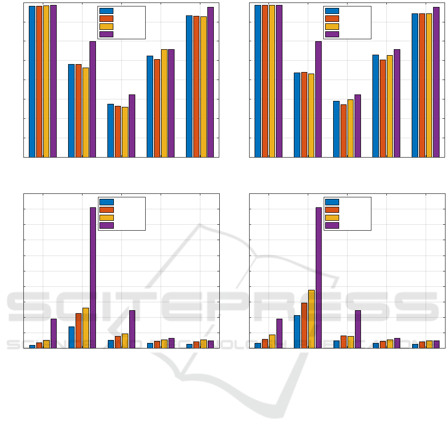
In Figure 1, we compare the performances achieved

by the exhaustive procedure in terms of accuracy on

the test set (in percentage) and total wall-clock time

(in minutes) against the proposed subsampling proce-

dures. Due to the intrinsic randomness in the training

procedures, results herein presented have been aver-

aged across ﬁve runs. The random extraction proce-

dure has been tested with three different values of W ,

up to a maximum subgraph order o. It is notewor-

thy that aim of our analyses is to investigate on how

the subsampling rate impacts on accuracy, memory

footprint and running times: as such, all parameters

except W itself have been kept constant.

By matching Figures 1a and 1b, it is possible to

see that the novel strategies lead to comparable re-

sults (in terms of accuracy) with those obtained by

the exhaustive procedure for every value of W . The

only remarkable shift can be observed for GREC (ap-

proximately 5%). It is worth remarking that the per-

formances of the classiﬁcation block are strongly in-

ﬂuenced by the efﬁciency of the mapping function

in preserving the graph input space properties into

the R

space. This can be achieved only if the in-

formation granules extracted are indeed meaningful

representatives of the considered dataset(s). For all

datasets, clearly some properties emerge even by per-

forming a strong subsampling of the prospective sub-

graphs.

Other than comparable results in terms of accu-

racy, remarkable improvements in terms of running

time can be observed as well (Figures 1c and 1d).

This is due to the lower number of subgraphs returned

by the Extractor driving mainly the Granulator and

due to the traverse strategy adopted by the Embed-

der before the evaluation of the symbolic histograms.

Recalling Section 3.5.1, the genetic algorithm must

repeat several times the entire procedure of granula-

tion, embedding and classiﬁcation in order to opti-

mize the parameters involved. This task involves the

GED computation many times, which can be very in-

tensive and time consuming. By matching Table 1

and Figures 1c–1d, clearly the advantages of subsam-

pling are more and more evident as the dataset size

increases and/or in presence of complex semantic in-

formation on nodes/edges, as their dissimilarity mea-

sures impact the overall GED computational burden.

5 CONCLUSIONS

In this paper, we addressed the possibility of design-

ing a Granular Computing-based classiﬁcation system

for labelled graphs by performing stochastic extrac-

tion procedures on the training data in order to im-

Stochastic Information Granules Extraction for Graph Embedding and Classiﬁcation

399

AIDS GREC Letter-H Letter-M Letter-L

100

Accuracy [%]

W = 10%

W = 30%

W = 50%

Exhaustive

(a) Accuracy on the Test Set (BFS)

AIDS GREC Letter-H Letter-M Letter-L

100

Accuracy [%]

W = 10%

W = 30%

W = 50%

Exhaustive

(b) Accuracy on the Test Set (DFS)

AIDS GREC Letter-H Letter-M Letter-L

100

120

140

160

180

200

Time [min]

W = 10%

W = 30%

W = 50%

Exhaustive

AIDS GREC Letter-H Letter-M Letter-L

100

120

140

160

180

200

Time [min]

W = 10%

W = 30%

W = 50%

Exhaustive

(d) Overall Running Time (DFS)

Figure 1: Comparison between the exhaustive procedure and the proposed stochastic sampling.

prove the information granulation procedure both in

terms of running time and memory footprint. The hy-

pothesis behind a stochastic granulation procedure is

that the information (regularities), whether present in

the dataset, can still be observed if subsamples of the

dataset itself are considered. In plainer words, mean-

ingful clusters are still visible.

In order to prove this concept, we equipped

GRALG with a different granulation procedure that

instead of ﬁnding information granules on the en-

tire set of possible subgraphs, such subgraphs are

extracted by performing stochastic extraction proce-

dures driven by well-known graph traversing algo-

rithms, namely DFS and BFS. These two strategies

are also considered when building the embedding

space, since the symbolic histograms paradigm relies

on counting how many times the symbols from the al-

phabet appear in the original graphs. Indeed, DFS and

BFS have been used to traverse the input graphs and

match the resulting subgraphs with the alphabet.

This lightweight procedure for extracting sub-

graphs both at granulation stage and at embedding

stage drastically outperforms the former exhaustive

procedure in terms of memory footprint and running

times and, at the same time, results in terms of accu-

racy on the test set are comparable with respect to the

former case. The achieved results somehow prove our

hypothesis, at least for the considered datasets, show-

ing that clustering techniques may be promising for

synthesizing information granules even with random

subsampling. This is particularly crucial in Big Data

scenarios, where the memory footprint is a delicate

issue and where redundancies and noisy patterns can

easily be found in massive datasets.

Nonetheless, the overall system keeps the pe-

culiar properties typical of information granulation-

NCTA 2019 - 11th International Conference on Neural Computation Theory and Applications

400

based systems, namely the human-interpretability of

the synthesized model. Indeed, the resulting informa-

tion granules can give insights to ﬁeld-experts about

the modelled system. This aspect is stressed by the

second genetic optimization, which is in charge of

shrinking the alphabet size, hence ﬁnding the subset

of information granules better related to the semantic

behind the classiﬁcation problem at hand.

As already mentioned, subsampling procedures

are appealing especially in Big Data scenarios. As

such, future research avenues can consider the im-

plementation of the proposed alphabet synthesis tech-

niques in parallel and distributed frameworks (Dean

and Ghemawat, 2008; Zaharia et al., 2010), even-

tually following multi-agent paradigms (Cao et al.,

2009; Altilio et al., 2019), or by means of dedicated

hardware (Tran et al., 2016; Cinti et al., 2019) in or-

der to properly face massive datasets and/or datasets

with non-trivial semantic information on both nodes

and edges. Thanks to these paradigms, the dataset can

be shred across several computational units and, most

importantly, the GED evaluation can be performed in

parallel, being it the most computationally expensive

step in the synthesis procedure.

REFERENCES

Altilio, R., Di Lorenzo, P., and Panella, M. (2019). Dis-

tributed data clustering over networks. Pattern Recog-

nition, 93:603 – 620.

Bai, X. (2012). Graph-Based Methods in Computer Vision:

Developments and Applications: Developments and

Applications. IGI Global.

Bargiela, A. and Pedrycz, W. (2006). The roots of granular

computing. In 2006 IEEE International Conference

on Granular Computing, pages 806–809.

Bargiela, A. and Pedrycz, W. (2008). Toward a theory

of granular computing for human-centered informa-

tion processing. IEEE Transactions on Fuzzy Systems,

16(2):320–330.

Bianchi, F. M., Livi, L., Rizzi, A., and Sadeghian, A.

(2014a). A granular computing approach to the de-

sign of optimized graph classiﬁcation systems. Soft

Computing, 18(2):393–412.

Bianchi, F. M., Scardapane, S., Livi, L., Uncini, A., and

Rizzi, A. (2014b). An interpretable graph-based im-

age classiﬁer. In 2014 International Joint Conference

on Neural Networks (IJCNN), pages 2339–2346.

Bianchi, F. M., Scardapane, S., Rizzi, A., Uncini, A.,

and Sadeghian, A. (2016). Granular computing tech-

niques for classiﬁcation and semantic characterization

of structured data. Cognitive Computation, 8(3):442–

461.

Bunke, H. (1997). On a relation between graph edit distance

and maximum common subgraph. Pattern Recogni-

tion Letters, 18(8):689 – 694.

Bunke, H. (2000). Graph matching: Theoretical founda-

tions, algorithms, and applications. In Proceedings of

Vision Interface, pages 82–88.

Bunke, H. (2003). Graph-based tools for data mining and

machine learning. In Perner, P. and Rosenfeld, A., ed-

itors, Machine Learning and Data Mining in Pattern

Recognition, pages 7–19, Berlin, Heidelberg. Springer

Berlin Heidelberg.

Bunke, H. and Allermann, G. (1983). Inexact graph match-

ing for structural pattern recognition. Pattern Recog-

nition Letters, 1(4):245 – 253.

Cao, L., Gorodetsky, V., and Mitkas, P. A. (2009). Agent

mining: The synergy of agents and data mining. IEEE

Intelligent Systems, 24(3):64–72.

Cinti, A., Bianchi, F. M., Martino, A., and Rizzi, A. (2019).

A novel algorithm for online inexact string matching

and its fpga implementation. Cognitive Computation.

Cortes, C. and Vapnik, V. (1995). Support-vector networks.

Machine learning, 20(3):273–297.

Cover, T. M. and Hart, P. E. (1967). Nearest neighbor pat-

tern classiﬁcation. IEEE Transactions on Information

Theory, 13(1):21–27.

Dean, J. and Ghemawat, S. (2008). Mapreduce: simpliﬁed

data processing on large clusters. Communications of

the ACM, 51(1):107–113.

Del Vescovo, G., Livi, L., Frattale Mascioli, F. M., and

Rizzi, A. (2014). On the problem of modeling struc-

tured data with the minsod representative. Interna-

tional Journal of Computer Theory and Engineering,

6(1):9.

Del Vescovo, G. and Rizzi, A. (2007a). Automatic classi-

ﬁcation of graphs by symbolic histograms. In 2007

IEEE International Conference on Granular Comput-

ing (GRC 2007), pages 410–416. IEEE.

Del Vescovo, G. and Rizzi, A. (2007b). Online handwrit-

ing recognition by the symbolic histograms approach.

In 2007 IEEE International Conference on Granular

Computing (GRC 2007), pages 686–686. IEEE.

Di Noia, A., Martino, A., Montanari, P., and Rizzi, A.

(2019). Supervised machine learning techniques and

genetic optimization for occupational diseases risk

prediction. Soft Computing.

Di Paola, L. and Giuliani, A. (2017). Protein–Protein Inter-

actions: The Structural Foundation of Life Complex-

ity, pages 1–12. American Cancer Society.

Ding, S., Du, M., and Zhu, H. (2015). Survey on granularity

clustering. Cognitive neurodynamics, 9(6):561–572.

Ghosh, S., Das, N., Gonçalves, T., Quaresma, P., and

Kundu, M. (2018). The journey of graph kernels

through two decades. Computer Science Review,

27:88–111.

Giuliani, A., Filippi, S., and Bertolaso, M. (2014). Why

network approach can promote a new way of thinking

in biology. Frontiers in Genetics, 5:83.

Han, J. and Lin, T. Y. (2010). Granular computing: Models

and applications. International Journal of Intelligent

Systems, 25(2):111–117.

Howard, N. and Lieberman, H. (2014). Brainspace: Re-

lating neuroscience to knowledge about everyday life.

Cognitive Computation, 6(1):35–44.

Stochastic Information Granules Extraction for Graph Embedding and Classiﬁcation

401

Krishnan, A., Zbilut, J. P., Tomita, M., and Giuliani, A.

(2008). Proteins as networks: usefulness of graph the-

ory in protein science. Current Protein and Peptide

Science, 9(1):28–38.

Livi, L., Del Vescovo, G., Rizzi, A., and Frattale Mas-

cioli, F. M. (2014). Building pattern recognition

applications with the spare library. arXiv preprint

arXiv:1410.5263.

Livi, L. and Sadeghian, A. (2016). Granular comput-

ing, computational intelligence, and the analysis of

non-geometric input spaces. Granular Computing,

1(1):13–20.

Martino, A., Giuliani, A., and Rizzi, A. (2018a). Gran-

ular computing techniques for bioinformatics pat-

tern recognition problems in non-metric spaces. In

Pedrycz, W. and Chen, S.-M., editors, Computational

Intelligence for Pattern Recognition, pages 53–81.

Springer International Publishing, Cham.

Martino, A., Rizzi, A., and Frattale Mascioli, F. M. (2017).

Efﬁcient approaches for solving the large-scale k-

medoids problem. In Proceedings of the 9th Inter-

national Joint Conference on Computational Intelli-

gence - Volume 1: IJCCI,, pages 338–347. INSTICC,

SciTePress.

Martino, A., Rizzi, A., and Frattale Mascioli, F. M. (2018b).

Distance matrix pre-caching and distributed computa-

tion of internal validation indices in k-medoids clus-

tering. In 2018 International Joint Conference on

Neural Networks (IJCNN), pages 1–8.

Martino, A., Rizzi, A., and Frattale Mascioli, F. M.

(2019). Efﬁcient approaches for solving the large-

scale k-medoids problem: Towards structured data.

In Sabourin, C., Merelo, J. J., Madani, K., and War-

wick, K., editors, Computational Intelligence: 9th In-

ternational Joint Conference, IJCCI 2017 Funchal-

Madeira, Portugal, November 1-3, 2017 Revised Se-

lected Papers, pages 199–219. Springer International

Publishing, Cham.

Neuhaus, M. and Bunke, H. (2007). Bridging the gap be-

tween graph edit distance and kernel machines, vol-

ume 68. World Scientiﬁc.

Pedrycz, W. (2005). Knowledge-based clustering: from

data to information granules. John Wiley & Sons.

Pedrycz, W. (2010). Human centricity in computing with

fuzzy sets: an interpretability quest for higher order

granular constructs. Journal of Ambient Intelligence

and Humanized Computing, 1(1):65–74.

Pedrycz, W. (2013). Proximity-based clustering: a search

for structural consistency in data with semantic blocks

of features. IEEE Transactions on Fuzzy Systems,

21(5):978–982.

Pedrycz, W. (2016). Granular computing: analysis and de-

sign of intelligent systems. CRC press.

Pedrycz, W. and Homenda, W. (2013). Building the

fundamentals of granular computing: A principle

of justiﬁable granularity. Applied Soft Computing,

13(10):4209 – 4218.

P˛ekalska, E. and Duin, R. P. (2005). The dissimilarity rep-

resentation for pattern recognition: foundations and

applications.

Richiardi, J., Achard, S., Bunke, H., and Van De Ville, D.

(2013). Machine learning with brain graphs: predic-

tive modeling approaches for functional imaging in

systems neuroscience. IEEE Signal Processing Mag-

azine, 30(3):58–70.

Riesen, K. and Bunke, H. (2008). Iam graph database

repository for graph based pattern recognition and ma-

chine learning. In Joint IAPR International Work-

shops on Statistical Techniques in Pattern Recognition

(SPR) and Structural and Syntactic Pattern Recogni-

tion (SSPR), pages 287–297. Springer.

Theodoridis, S. and Koutroumbas, K. (2008). Pattern

Recognition. Academic Press, 4 edition.

Tran, H.-N., Cambria, E., and Hussain, A. (2016). Towards

gpu-based common-sense reasoning: Using fast sub-

graph matching. Cognitive Computation, 8(6):1074–

1086.

Tsai, W.-H. and Fu, K.-S. (1979). Error-correcting isomor-

phisms of attributed relational graphs for pattern anal-

ysis. IEEE Transactions on systems, man, and cyber-

netics, 9(12):757–768.

Vishwanathan, S. V. N., Schraudolph, N. N., Kondor, R.,

and Borgwardt, K. M. (2010). Graph kernels. Journal

of Machine Learning Research, 11(Apr):1201–1242.

Wang, F. and Sun, J. (2015). Survey on distance metric

learning and dimensionality reduction in data mining.

Data Mining and Knowledge Discovery, 29(2):534–

564.

Wang, G., Yang, J., and Xu, J. (2017). Granular

computing: from granularity optimization to multi-

granularity joint problem solving. Granular Comput-

ing, 2(3):105–120.

Weinshall, D., Jacobs, D. W., and Gdalyahu, Y. (1999).

Classiﬁcation in non-metric spaces. In Kearns, M. J.,

Solla, S. A., and Cohn, D. A., editors, Advances

in Neural Information Processing Systems 11, pages

838–846. MIT Press.

Yang, J., Wang, G., and Zhang, Q. (2018). Knowledge

distance measure in multigranulation spaces of fuzzy

equivalence relations. Information Sciences, 448:18–

35.

Yao, Y. (2016). A triarchic theory of granular computing.

Granular Computing, 1(2):145–157.

Yao, Y. and Zhao, L. (2012). A measurement theory view

on the granularity of partitions. Information Sciences,

213:1–13.

Yao, Y.-Y. (2008). The rise of granular computing. Journal

of Chongqing University of Posts and Telecommuni-

cations (Natural Science Edition), 20(3):299–308.

Zadeh, L. A. (1979). Fuzzy sets and information granu-

larity. Advances in fuzzy set theory and applications,

11:3–18.

Zadeh, L. A. (1997). Toward a theory of fuzzy information

granulation and its centrality in human reasoning and

fuzzy logic. Fuzzy sets and systems, 90(2):111–127.

Zaharia, M., Chowdhury, M., Franklin, M. J., Shenker, S.,

and Stoica, I. (2010). Spark: Cluster computing with

working sets. In Proceedings of the 2nd USENIX

Conference on Hot Topics in Cloud Computing, Hot-

Cloud’10, pages 10–10. USENIX Association.

NCTA 2019 - 11th International Conference on Neural Computation Theory and Applications

402