LOS/NLOS Wireless Channel Identiﬁcation based on Data Mining of

UWB Signals

Gianluca Moro

, Roberto Pasolini

and Davide Dardari

Department of Computer Science and Engineering - DISI, University of Bologna,

Via dell’Universit

a 50, I-47522 Cesena (FC), Italy

Department of Electrical, Electronic and Information Engineering – DEI, University of Bologna,

Via dell’Universit

a 50, I-47522 Cesena (FC), Italy

Keywords: Ultra-Wide Band, Localization, Non-Line-Of-Sight Identiﬁcation, Data Mining, Machine Learning.

Abstract:

Localisation algorithms based on the estimation of the time-of-arrival of the received signal are particularly

interesting when ultra-wide band (UWB) signaling is adopted for high-deﬁnition location aware applications.

In this context non-line-of-sight (NLOS) propagation condition may drastically degrade the localisation accu-

racy if not properly recognised. We propose a new NLOS identiﬁcation technique based on the analysis of

UWB signals through supervised and unsupervised machine learning algorithms, which are typically adopted

to extract knowledge from data according to the data mining approach. Thanks to these algorithms we can

automatically generate a very reliable model that recognises if an UWB received signal has crossed obstacles

(NLOS situation). The main advantage of this solution is that it extracts the model for NLOS identiﬁcation

directly from example waveforms gathered in the environment and does not rely on empirical tuning of param-

eters as required by other NLOS identiﬁcation algorithms. Moreover experiments show that accurate NLOS

classiﬁers can be extracted from measured signals either pre-classiﬁed or unclassiﬁed and even from samples

algorithmically-generated from statistical models, allowing the application of the method in real scenarios

without training it on real data.

1 INTRODUCTION

Location awareness in wireless networks is becom-

ing essential for commercial and military applica-

tions, especially in data-centric and Internet of every-

thing (IoE) sensor networks (Moro and Monti, 2012),

where can be used to seamlessly query and collect

spatially-located big data, or in real-time locating sys-

tems (Tseng et al., 2001; Cheng et al., 2012). One

of the most important approaches to estimate location

of wireless systems is based on time-of-arrival (TOA)

estimation of received radio signals (Li and Pahla-

van, 2004; Alsindi et al., 2004; Dardari et al., 2015).

When adopted in association with the ultra-wide band

(UWB) technology, a high accuracy in ranging can be

potentially retrieved (Lagunas et al., 2010).

However, in harsh environments, such as indoor,

the presence of obstacles usually degrades signiﬁ-

cantly the ranging performance, as the direct path

might be blocked or delayed and ranging information

is derived from reﬂected paths. This leads to over-

estimation of distances and subsequently to a faulty

localisation (Denis et al., 2003; Dardari et al., 2009).

A common approach to deal with this problem

is to identify non-line-of-sight (NLOS) situations

among received waveforms and apply some sort of

correction, such as reducing or removing their inﬂu-

ence in determining receiver position. Many concrete

solutions have been proposed in literature, which are

generally based on recognising NLOS situations from

known peculiarities of the measured waveforms, as

will be detailed in Sec. 2.2.

These methods and their accuracy depend gener-

ally from a time-consuming tuning phase of param-

eters, which are set empirically according to the en-

vironment. Moreover, methods are usually tuned and

tested on speciﬁc environments, leading them to be

optimised only for those particular scenarios. For

these reasons, the application of these solutions to dif-

ferent environments require each time costly human

interventions.

An approach to overcome these limits is to iden-

tify NLOS signals using a knowledge model which

should be directly extracted from the application en-

416

Moro, G., Pasolini, R. and Dardari, D.

LOS/NLOS Wireless Channel Identiﬁcation based on Data Mining of UWB Signals.

DOI: 10.5220/0008119504160425

In Proceedings of the 8th International Conference on Data Science, Technology and Applications (DATA 2019), pages 416-425

ISBN: 978-989-758-377-3

vironment through an automated process.

Data mining process involves the extraction of

non-trivial information from large volumes of data

(Fayyad et al., 1996; Han et al., 2006; Hastie et al.,

2005; Domeniconi et al., 2015b; Domeniconi et al.,

2014a; di Lena et al., 2015). Summarily, this process

involves the transformation of “raw” available data

into a speciﬁc structured form, which is given in in-

put to machine learning algorithms to obtain general

knowledge models describing the data. For our pur-

poses, after observing the propagation of some con-

trolled signals in the target environment, we can em-

ploy an automated procedure using these techniques

to generalise these observations into a model, allow-

ing to make assumptions on subsequently observed

signals; more speciﬁcally, to identify them as either

line-of-sight (LOS) or NLOS.

This approach has been applied for example in

(Marano et al., 2010), where least-squares support

vector machines (Suykens et al., 2002; Nguyen et al.,

2015) are employed to distinguish between LOS and

NLOS situations and also to mitigate the positive bi-

ases present in NLOS range estimates. This is an ex-

ample of supervised learning, such as in (Choi et al.,

2018) that is based on novel deep learning approaches

but using WLAN signals that achieve a lower accu-

racy than UWB channels.

These supervised methods require a set of wave-

form examples which must be a-priori manually la-

belled as LOS or NLOS: the learning algorithm ex-

tracts non-trivial distinctive patterns of these two

classes into a model, used to classify subsequent sig-

nals as either LOS or NLOS. An important limit of

supervised learning is the need for labelled examples:

a notable amount of human work is generally required

to collect and classify a number of waveforms sufﬁ-

cient to obtain an accurate model.

In this work we investigate further data mining-

based solutions for the identiﬁcation of NLOS wave-

forms. Notably, other than supervised learning, we

also test the use of unsupervised learning (Cerroni

et al., 2015), where knowledge is extracted from un-

labelled example waveforms, that is without requiring

their costly pre-classiﬁcation by human experts. Un-

supervised algorithms discover heterogeneous groups

made up of homogeneous data, whose distinctive

traits can be easily connected to either LOS or NLOS

situation. As the example waveforms do not need to

be pre-classiﬁed by experts, i.e. labelled, the con-

struction of an usable training dataset is straightfor-

ward and inexpensive.

We evaluate different supervised and unsuper-

vised learning algorithms, known to yield fairly accu-

rate models in many practical situations, despite hav-

ing relatively trivial implementations and fast execu-

tion times. This makes them good candidates for be-

ing deployed and run directly on radio equipment or

other resource-limited embedded devices. By testing

the proposed methods on benchmark data constituted

of both measured and simulated signals, we demon-

strate that the proposed approaches are fairly good

in distinguishing LOS waveforms from NLOS ones.

This potentially guarantees accurate localisation by

applying algorithms like that proposed in (Marano

et al., 2010) on multiple waveforms. Models tested

on real measured waveforms prove to be reliable even

when built from unlabelled signals or from wave-

forms generated by statistical models, thus making

the training process in real use cases more straight-

forward.

In Section 2, we ﬁrst introduce the application

context, in order to motivate the need for NLOS iden-

tiﬁcation; methods proposed in literature are revised

thereafter. Then, in Section 3 we present our solution,

indicating the high-level procedure, how feature vec-

tors are obtained from signals and which algorithms

we adopted for their analysis. Finally, in Sections 4

and 5 we report the evaluation of the proposed solu-

tion, describing the data used as benchmark and re-

porting and discussing the accuracy measured from

the tested methods. Section 6 sums up the work and

suggests future directions.

2 NLOS IDENTIFICATION FOR

LOCALISATION

2.1 Localisation using Ranging

Measurements

Here we summarise the process of localisation

through UWB signals, in order to motivate the impor-

tance of distinguishing NLOS situations when max-

imising the localisation accuracy.

We picture a typical reference scenario with a

moving agent with an unknown position p and a set of

anchors with known ﬁxed positions p

,... ,p

. Using

a ranging protocol, the agent can obtain an estimation

of the effective distance d

= kp − p

k from each

station, characterised by a ranging error ε

− d

Information about position and distance of at least

three stations can be used to compute an estimation

p of the agent position in 2D, for example by means

of the least squares criterion

p = argmin

∑

i=1



−

p − p



LOS/NLOS Wireless Channel Identiﬁcation based on Data Mining of UWB Signals

417

A complete discussion of ranging protocols is

given in (Sahinoglu et al., 2011), while a recent sur-

vey on further approaches can be found in (Dardari

et al., 2015). In order to obtain an accurate local-

isation, ranging errors must be as small as possible

and eventually unbiased. Effects like thermal noise

and multipath propagation inﬂuence on the distance

estimation accuracy. If the direct path between the

two points is obstructed by a wall or other obstacles,

we have so-called NLOS propagation: the distance

will be overestimated due to either reduced propaga-

tion speed through material or measurement of a re-

ﬂected path in case of complete obstruction. This phe-

nomenon has far more impact than other effects cited

above and can lead to important errors in the ﬁnal po-

sition estimation (Dardari et al., 2009).

However, if we are able to identify which signals

correspond to NLOS situations among those used to

estimate position, we can apply some form of cor-

rection to the estimation procedure in order to im-

prove its accuracy. For example, when using the least

squares criterion, NLOS signals could be weighted

with a lower value in the cost function to be min-

imised.

In the following, we speciﬁcally focus on the

problem of analysing single waveforms in order to

distinguish NLOS situations. The proposed solutions

can be plugged in a localisation algorithm as proposed

in (Marano et al., 2010) or in any other suitable con-

text.

2.2 Related Work on NLOS Detection

Different approaches have been proposed to recognise

NLOS propagation in UWB signals.

In (Wylie and Holtzman, 1996) the measurement

noise variance is assumed to be known and the stan-

dard deviation of ranging measurements is compared

with an empirical threshold to identify LOS/NLOS

situations. In (Borras et al., 1998) it is presented a

statistical approach based on the availability of a pri-

ori information about the environment, such as the

probability density function (PDF) of the TOA mea-

surements: all ﬁve proposed methods are based on

the fact that measurements variation in NLOS situa-

tions is much higher than in LOS ones; the thresh-

old, however, strongly depends on the particular sta-

tistical model adopted. An approach where a suitable

distance metric is used between the known measure-

ment error distribution and the non-parametrically es-

timated distance measurement distribution in order to

classify a measurement as in LOS or NLOS condi-

tion is discussed in (Gezici et al., 2003). Interesting

results have been also obtained by Guvenc et al. in

(Guvenc et al., 2007) where they propose four differ-

ent solutions for the classiﬁcation problem of signals

generated by standard models (Molisch et al., 2006),

everyone based on a ratio between various PDF al-

ways compared with a ﬁxed threshold.

Given the variety of measurement conditions and

the recurring need to tune parameters, more recent

methods propose to exploit known waveforms to learn

optimal parameters. In (Decarli et al., 2010) is pro-

posed to use a set of waveforms to estimate param-

eters for likelihood estimation of LOS and NLOS

situations based on some key features. In (Marano

et al., 2010) the authors developed techniques to dis-

tinguish between LOS and NLOS situations, and to

mitigate the positive biases present in NLOS range

estimates. Their techniques are non-parametric and

are based on least-squares support vector machines

(LS-SVM) (Suykens et al., 2002), a supervised clas-

siﬁcation technique. In (M

uller et al., 2014) Gaussian

mixture ﬁlters are used for classiﬁcation.

Recent approaches also exist which perform lo-

calisation by exploiting multipath propagation rather

than ﬁltering it out: they are not as accurate as classic

trilocation-based methods, but are suitable to situa-

tions where a single ﬁxed station is available (Kuang

et al., 2013; Zhu et al., 2015).

3 NLOS IDENTIFICATION

THROUGH DATA MINING

Data Mining (DM), also known as Knowledge Dis-

covery on Databases (KDD), is deﬁned as the process

of discovering non-trivial patterns in data (Witten and

Frank, 2005). These discovery processes must be au-

tomatic or, at least, semiautomatic, when a human in-

teraction is needed, especially in the ﬁrst steps of the

process. Data are almost always in an electronic form

stored in one or many databases.

Before applying algorithms to discover patterns,

the target dataset must be large enough to contain

these patterns while remaining concise enough to

be mined in an acceptable timeframe. In the pre-

processing phase, the target dataset is created – if nec-

essary – and reduced into feature vectors, one vector

per observation. A feature vector, often called in-

stance, is a summarised version of the raw data ob-

servation, composed of its most signiﬁcant features.

A set of such vectors can be fed into input to a

learning algorithm, which treats them as examples to

extract underlying patterns within them and encap-

sulate them in a representative data model. Many

learning algorithms exist, based on different theoret-

ical bases and yielding models of different formats.

DATA 2019 - 8th International Conference on Data Science, Technology and Applications

418

We consider here two different major approaches to

learning, differing in the nature of input data.

Supervised learning algorithms. They take as in-

put labelled instances, i.e. each instance must be la-

belled with one of two or more possible classes, in-

dicating the characteristic of the instance we are in-

terested in. The resulting model describes the typical

patterns of each distinct class and can be used to in-

fer the most likely class of any other instance. In our

case, waveform instances are labelled as either LOS

or NLOS, such that the ﬁnal model is able to classify

subsequent pre-processed waveforms in one of these

two cases.

Unsupervised learning. On the other side these

algorithms take unlabelled instances as input, with

no additional information. These algorithms parti-

tion given instances into clusters, i.e. heterogeneous

groups of homogeneous instances. The goal of these

algorithms is both to maximise the similarity between

instances of a same cluster and to minimise instead

that between instances of different clusters. As a re-

sult, each cluster will contain instances with speciﬁc

prominent characteristics, which can be easily linked

to high-level phenomenons we are trying to observe.

In our case, we can provide a huge quantity of unla-

belled waveforms to a clustering algorithm in order

to obtain a small number of clusters, which can be

labelled as either LOS or NLOS with minimal effort.

The advantage of the supervised learning ap-

proach is that it is speciﬁcally ﬁtted for the classi-

ﬁcation problem and usually yields a more accurate

model of the aspect we are interested in, in this case

being the NLOS propagation. On the other side, the

unsupervised approach yields a more generic model

which subdivides instances in groups with no prede-

ﬁned meaning, but these groups can potentially be

easily mapped to either LOS or NLOS situations and

the accuracy is in some cases nearly as good as that

obtained by supervised learning.

In the following, we ﬁrst describe how we pre-

process each waveform to extract a set of predictive

features, then we discuss the speciﬁc supervised and

unsupervised learning methods taken into considera-

tion for knowledge extraction.

3.1 Feature Selection from Raw Data

The ﬁrst step is to get the relevant attributes from the

waveforms we expect to be affected by the NLOS

condition, in order to have records with signiﬁcative

features.

After reducing each waveform to its single sam-

ples, we initially chose to directly use the values of

such samples as attributes. This choice leads in gen-

eral to a very large number of attributes, which is not

a favourable situation for DM algorithms. To avoid

this situation, some form of data aggregation is rec-

ommended: its former advantage is the reduction of

the attributes number, but this elaboration is useful

also to extract new possible signiﬁcant data from the

raw signal.

The N samples of each waveform are divided into

windows, composed of W points each. Then for each

window we choose M derived attributes. In this way

we obtain F attributes:

F =

M · N

Each window is in practice a sequence of values

x = (x

,. .. ,x

), with n =

being the resulting num-

ber of points per window. In Table 1 we present the

statistics that we used as attributes for each window.

In particular, skewness is a measure of the lack of

symmetry in a data set. A data set, or distribution,

is symmetric if it looks the same to the left and right

of the center point. Kurtosis instead is a measure of

whether the data are peaked or ﬂat relative to a normal

distribution. That is, data sets with high kurtosis tend

to have a distinct peak near the mean, decline rather

rapidly, and have heavy tails. Data sets with low kur-

tosis tend to have a ﬂat top near the mean rather than

a sharp peak.

The formulas for skewness b

and kurtosis g

are:

∑

i=1

− ¯x)

(n − 1)s

∑

i=1

− ¯x)

(n − 1)s

where ¯x is the mean, s is the standard deviation,

and n is the number of data points.

The energy of the signals is calculated on ﬁxed

size disjointed windows; for each window, the value

is:

E =

∑

i=1

It is possible, depending of the situation, to use

other many different attributes focusing in particular

on aggregated attributes, derived from the combina-

tion of other ones.

During the training phase in supervised algo-

rithms, the correct class – LOS or NLOS – is associ-

ated to each waveform. Whereas the ﬁrst step do not

depend on which kind of data mining algorithms we

are going to use, this labelling step is not necessary if

we are going to use clustering algorithms. Clusterers

are unsupervised so do not need classiﬁed instances to

LOS/NLOS Wireless Channel Identiﬁcation based on Data Mining of UWB Signals

419

Table 1: Attributes calculated from waveform signal points for each window.

Max maximum value x

Max

min minimum value x

min

Absolute Max maximum absolute value |x|

Max

Absolute min minimum absolute value |x|

min

Mean mean value for the window ¯x

Std. deviation distribution’s standard deviation s

Skewness distribution’s skewness b

Kurtosis distribution’s kurtosis g

Energy signal’s part energy E

Max / min ratio between Max and min values x

Max

min

Max - min difference between Max and min values x

Max

− x

min

SD / mean ratio between std. deviation and mean s/¯x

Max - min sqrd. squared difference between Max and min (x

Max

− x

min

)

generate the model, they divide data into groups with-

out knowing the correct class. However, to evaluate

the performance of these algorithms, we need to com-

pared the produced clusters with the instances’ class

value.

3.2 Bayesian Network

The probabilistic approach to automated classiﬁca-

tion entails to estimate from the training set the con-

ditional probabilities of each possible class according

to the values of predictive features, hence referred to

as variables. A trivial application of this principle

is the Na

ıve Bayes classiﬁer, which assumes mutual

conditional independence between all variables: con-

sidering the Bayes’ theorem, the posterior probability

P(c|x) of an instance x to represent a class c can be

computed as a product of conditional probabilities for

each variable x

,. .. (Lewis, 1998).

P(c|x) ∝ P(c) · P(x|c)

∼

P(c) · P(x

|c) · P(x

|c) · ...

In order to account for existing conditional de-

pendencies between variables, we employ Bayesian

networks as classiﬁcation models. Such a network is

deﬁned by a directed acyclic graph on variables, indi-

cating their conditional dependencies; to each node of

the graph is associated a conditional probability table

on possible values of the corresponding variable, con-

ditioned by values of parent variables (Pearl, 2014).

Once the network structure is deﬁned, probability ta-

bles for each node can be trivially estimated from the

training data. Moreover, various methods exist to au-

tomatically learn even the graph itself from data, e.g.

by means of local search algorithms. Use of such ta-

bles requires to work with discrete variables: contin-

uous ones need to be converted e.g. by binning.

While the construction of an optimal dependency

graph can be cumbersome, depending on the speciﬁc

method used, the calculation of probability tables and

their subsequent use for classiﬁcation are straightfor-

ward.

3.3 C4.5 Decision Trees

A decision tree-based classiﬁcation model is consti-

tuted by a rooted tree where each intermediate node

corresponds to a feature and its outgoing edges corre-

spond to its possible values. To classify an instance,

starting from the root node, one must recursively fol-

low the edge labelled with the value of the current fea-

ture, until a leaf node indicating the most likely class

is reached.

C4.5 (Quinlan, 1993) is one of the most known

algorithms to learn a decision tree by examples. The

training set is split into groups according to the fea-

ture which better discriminates instances of different

classes and a tree node labelled with the same fea-

ture is created. This process is repeated recursively

on each split to generate the subtrees, stopping when

limit cases are met, such as when all instances of the

split are labelled with the same class. Discriminative

power of features is determined by means of informa-

tion entropy or related measures.

This is one of the most straightforward algorithms

for decision tree learning, yet it is able to yield fairly

accurate classiﬁers in many circumstances.

3.4 K-means

For the unsupervised learning approach, we con-

sider the well-known k-means algorithm (Hartigan

and Wong, 1979), which takes as parameter the num-

ber k of clusters to be generated. Each cluster is char-

acterised by a prototype vector, each instance is as-

DATA 2019 - 8th International Conference on Data Science, Technology and Applications

420

Figure 1: Map of the WiLAB showing the displacement of beacons (with “tx” labels) and targets across different rooms.

signed to the cluster having the closest prototype ac-

cording to the euclidean distance. After picking ran-

dom starting prototypes, the algorithm iteratively as-

sign each instance to the closest prototype and then

recalculates prototypes as the centroids (i.e. mean

points) of respective assigned instances, until all of

them converge to ﬁxed points. The goal of k-means is

to minimise the sum of squared distances between in-

stances of a same cluster, but the algorithm only guar-

antees convergence to a local optimum and can be

heavily inﬂuenced from the starting prototypes con-

ﬁguration.

4 EXPERIMENTAL SETUP

In order to assess the proposed data mining-based ap-

proach to distinguish LOS and NLOS propagation

cases, we set up an experimental evaluation process

aimed to estimate the accuracy of classiﬁers obtained

by using different combinations of selected features

and learning algorithms.

As a ﬁrst step for the validation of a mining model,

a consistent set of labelled instances accurately repre-

senting the target context must be collected. We used

two different datasets to this extent, which will be de-

scribed shortly.

Given a labelled dataset, the most straightforward

way to evaluate the process would be to train a clas-

siﬁcation model on the whole dataset and to check

whether for each instance it returns its correct class;

the accuracy would be given by the ratio of correctly

classiﬁed instances. However, evaluating a model us-

ing the same instances it was trained on is discour-

aged, as the capacity of the model to discover general

patterns and recognise them in previously unseen data

could not be properly assessed.

Instead, a common validation procedure is the k-

fold cross validation, where the dataset is split into k

complementary folds of equal size: instances of each

of them are used to evaluate a model trained on the re-

maining k −1 folds, the accuracy is then computed as

above and averaged across all folds. This guarantees

to test the approach on the whole dataset, yet avoiding

to test models on instances used for training.

The cross-validation is used to validate supervised

learning approaches. Instead, for unsupervised algo-

rithms, we compare the cluster assignment with the

real signal class. If the classes are not known a priori,

a valid measure of clustering performance is the sum

of squared errors within cluster: less is better.

For all the learning algorithms used, we relied

LOS/NLOS Wireless Channel Identiﬁcation based on Data Mining of UWB Signals

421

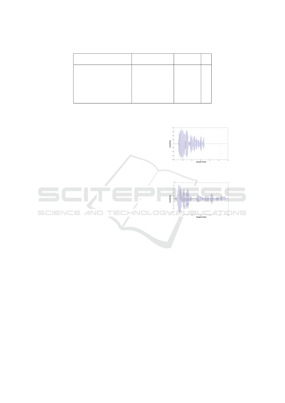
Table 2: Best accuracy of classiﬁcation and clustering for different sets of features.

Classiﬁcation Clustering

Attributes accuracy accuracy W

Each point (a) 86,72 % (Bayes) 75,52 % -

4 Attributes (b) 90,26 % (C4.5) 88,67 % 16

Energy 89,62 % (C4.5) 89,14 % 20

4 Attributes + Energy 90,26 % (C4.5) 88,66 % 16

Skewness + Kurtosis 87,19 % (Bayes) 70,08 % 16

Aggregated values (c) 88,79 % (C4.5) 12

4 Attributes + Aggr. Values 90,00 % (C4.5) 12

(a) Each point value used as attribute

(b) maximum, minimum, mean and standard deviation

upon their implementations available in WEKA, a

data mining framework written in Java (Hall et al.,

2009). Speciﬁcally, we used the BayesNet, J48 and

SimpleKMeans implementations provided with the

framework. In the case of k-means, we set the num-

ber of clusters k = 2, as the number of classes to be

recognised; for the rest, we used default values for all

parameters of each algorithm.

4.1 Datasets

For the evaluation process described above, we con-

sidered two different datasets of waveforms labelled

as either LOS or NLOS.

A ﬁrst dataset is composed of real waveforms ob-

tained from a measurement campaign whose full de-

tails are reported in (Dardari et al., 2008), conducted

at the WiLAB in University of Bologna (Italy), in a

typical ofﬁce indoor environment represented in Fig-

ure 1. Throughout the area, 5 UWB beacons were

deployed and 20 target positions were set. A com-

mercial UWB radio operating in the 3.2-7.4 GHz 10

dB RF bandwidth and arranged to perform ranging

by TOA estimation was placed at each target posi-

tion. 1,500 range measurements were taken for each

beacon-target couple and also for each pair of targets.

The chosen locations for beacons and targets are dis-

tributed across an hallway and rooms adjacent to it:

this gave a wide variety of both LOS and NLOS prop-

agation situations, with different effective distances

and obstacles inbetween. Obstacles are constituted

by concrete walls with thickness of either 15 cm or

30 cm and by typical ofﬁce furniture. Example of a

measured LOS signal is ploted in Figure 2.

A second dataset is instead composed of wave-

form signals generated algorithmically, according to

IEEE 802.15.4a (Molisch et al., 2006) statistical mod-

els for UWB channel, in particular from CM1 and

CM2 model for residential environments. Figure 3

shows an example of a LOS waveform, generated

Figure 2: Example of LOS signal from measured data (Dar-

dari et al., 2008).

Figure 3: Example of LOS signal using CM1 model.

through the CM1 model.

In the evaluation, by default we perform intra-

dataset experiments where the training and the test

set are extracted from the same dataset: this allows to

verify that classiﬁers are effectively able to correctly

handle instances extracted under the same conditions

of the training ones. In addition, we will also per-

form cross-dataset tests, where a model is trained on

a dataset and tested against instances of the other: in

this way, we verify whether the knowledge extracted

from one kind of waveforms can be applied seam-

lessly to the other one.

5 NUMERICAL RESULTS

As a ﬁrst step, we performed a large number of tests

in order to ﬁnd the best combination of settings re-

garding the extraction of vectors from the signals.

For this phase, we performed cross-validation on the

DATA 2019 - 8th International Conference on Data Science, Technology and Applications

422

Table 3: Model accuracy comparison intra-dataset (cross fold validation).

Training set Test set BayesNet C4.5 Cluster

Measured Measured 86,13% 88,45% 88,45%

Model (CM1, CM2) Model (CM1, CM2) 98,00% 95,50% 87,00%

Table 4: Results of the different methods presented in (Guvenc et al., 2007) for LOS and NLOS identiﬁcation.

Channel Model Kurtosis MED RMS-DS Joint

CM1 (Ofﬁce environment LOS) 78,6% 74,3% 61,7% 81,8%

CM2 (Ofﬁce environment NLOS) 83,2% 77,9% 76,1% 84,3%

Mean 80,9% 76,1% 68,9% 83,1%

Table 5: Model accuracy comparison inter-dataset

Training set Test set BayesNet C4.5 Cluster

Measured Model (CM1, CM2) 83,00% 72,5% 88,10%

Model (CM1, CM2) Measured 87,76% 85,69% 91,00%

measured signals dataset. Speciﬁcally, we considered

multiple subsets of features among those described

in Section 3.1, for each of them we then tested the

three discussed learning approaches by varying the

windows size W between 2 and 20.

Table 2 reports, for each subset of parameters, the

best accuracy results obtained for classiﬁcation and

clustering, along with the value of W that brought to

them.

By comparing the results for the different sets of

features, we notice that the most important ones for

prediction seem to be the four basic statistics maxi-

mum, minimum, mean and standard deviation, along

with the energy measure. On the contrary, using raw

sample values or more complex statistics by them-

selves we obtain a 2-3% lower accuracy in classiﬁ-

cation and a more remarkable gap in clustering. Re-

garding the learning algorithm to be used for classi-

ﬁcation, C4.5 turns out to usually be a better choice

than Bayesian networks.

As the four basic statistics, other than being com-

putable straightforwardly, seem to grant good accu-

racy levels, we will use them in the subsequent tests,

along with a window size W = 20. We report in Ta-

ble 3 the results obtained with these settings for each

learning algorithm applied to each of the two dataset,

with a suitable training-test set split.

Supervised classiﬁcation tests on the model-based

dataset brought substantially higher accuracy esti-

mates with respect to measured waveforms, while ac-

curacy levels for clustering are much closer. Results

on the model-based dataset can be compared with

those obtained by (Guvenc et al., 2007), reported in

Table 4.

Results in Table 3 lead to questioning whether the

higher accuracy on model-generated signals depends

from the test signals being more trivial to classify

or the model generated from the training signals be-

ing more accurate. More generally, we would like to

discover whether the model generated from one type

of signals – either measured or model-generated – is

general enough to be able to effectively classify sig-

nals of the other type. At this extent, further tests have

been run where a model is trained on one of the two

datasets and tested on the other one: results are re-

ported in Table 5.

While models trained on measured signals are not

as effective as in the previous cases in classifying

auto-generated signals, using the latter ones for train-

ing we achieved to build accurate classiﬁers for the

real signals. Supposedly, the use of regular model-

generated signals for training helps to build the classi-

ﬁer on the most informative signal features and avoids

to consider noise. Interestingly, this result suggests

that it is possible to accurately classify signals mea-

sured in a real, physical environment using a model

built on data which can be automatically generated

and labelled. In a real use case, the collection of

example waveforms to build the training set could

then be unnecessary: provided that suitable statistical

models for the considered environment exist, training

waveforms with similar features but noise-free can be

algorithmically generated.

6 CONCLUSIONS AND FUTURE

WORKS

In this paper, we presented a data mining-based ap-

proach to the recognition of NLOS propagation in

UWB signals, usable in localisation systems. Once

a set of example waveforms is collected, a knowledge

model can be extracted to classify further waveforms

in the same environment as either LOS or NLOS. We

LOS/NLOS Wireless Channel Identiﬁcation based on Data Mining of UWB Signals

423

employed a couple of supervised learning techniques

and also an unsupervised one, which does not require

training data to be labelled.

Taking a small indoor environment as reference,

experimental evaluation of the classiﬁcation accuracy

has been performed using datasets with both mea-

sured and simulated waveforms. Using waveforms

of the same type for training and test, the classiﬁca-

tion system achieves to outperform similar works in

literature, even in the unsupervised setting. More-

over, we obtained comparable or superior accuracy

levels when testing on real measured signals models

trained on simulated ones; this is a form of trans-

fer learning across different kinds of data which is

successfully adopted also in other data mining appli-

cation domains (Domeniconi et al., 2014b; Domeni-

coni et al., 2015a). On a general basis this can lead

to software/hardware applications able to achieve re-

liable classiﬁcation models trained on suitably sim-

ulated waveforms rather than from signal measured

each time from new target environments.

Future work may be aimed to further improve the

accuracy of the classiﬁcation models: many different

adjustments might be tested, including the use of new

features, for instance extracted from the frequency-

domain, or by weighting them according to their rele-

vance with approaches from other ﬁelds (Domeniconi

et al., 2016) or of different learning methods. Fur-

thermore, using the same features, regression algo-

rithms may be tested as done in (Marano et al., 2010)

to obtain effective weights of waveforms to use in lo-

calisation methods, rather than a binary LOS/NLOS

classiﬁcation. Concerning the scalability to a large

number of UWB emitters and receivers, this solution

can also be parallelized with peer-to-peer networks

of classiﬁers according to general purpose methods

like in (Cerroni et al., 2013) experimented in other

domains.

REFERENCES

Alsindi, N., Li, X., and Pahlavan, K. (2004). Perfor-

mance of TOA estimation algorithms in different in-

door multipath conditions. In Wireless Communica-

tions and Networking Conference, WCNC. IEEE, vol-

ume 1, pages 495–500. IEEE.

Borras, J., Hatrack, P., and Mandayam, N. B. (1998). Deci-

sion theoretic framework for NLOS identiﬁcation. In

Vehicular Technology Conference, 1998. VTC 98. 48th

IEEE, volume 2, pages 1583–1587. IEEE.

Cerroni, W., Moro, G., Pasolini, R., and Ramilli, M. (2015).

Decentralized Detection of Network Attacks Through

P2P Data Clustering of SNMP Data. Computers &

Security, 52:1–16.

Cerroni, W., Moro, G., Pirini, T., and Ramilli, M. (2013).

Peer-to-peer Data Mining Classiﬁers for Decentral-

ized Detection of Network Attacks. In Wang, H.

and Zhang, R., editors, Proceedings of the 24th Aus-

tralasian Database Conference, ADC 2013, volume

137 of CRPIT, pages 101–108, Darlinghurst, Aus-

tralia. Australian Computer Society, Inc.

Cheng, L., Wu, C., Zhang, Y., Wu, H., Li, M., and Maple,

C. (2012). A survey of localization in wireless sensor

network. International Journal of Distributed Sensor

Networks, 2012.

Choi, J., Lee, W., Lee, J., Lee, J., and Kim, S. (2018). Deep

learning based NLOS identiﬁcation with commodity

WLAN devices. IEEE Trans. Vehicular Technology,

67(4):3295–3303.

Dardari, D., Closas, P., and Djuric, P. M. (2015). Indoor

tracking: Theory, methods, and technologies. IEEE

Transactions on Vehicular Technology, 64(4):1263–

1278.

Dardari, D., Conti, A., Ferner, U., Giorgetti, A., and Win,

M. Z. (2009). Ranging with ultrawide bandwidth sig-

nals in multipath environments. Proceedings of the

IEEE, 97(2):404–426. Special Issue on UWB Tech-

nology & Emerging Applications.

Dardari, D., Conti, A., Lien, J., and Win, M. Z. (2008).

The effect of cooperation on localization systems us-

ing uwb experimental data. EURASIP Journal on Ad-

vances in Signal Processing, 2008.

Decarli, N., Dardari, D., Gezici, S., and D’Amico, A. A.

(2010). LOS/NLOS detection for UWB signals: A

comparative study using experimental data. In IEEE

5th International Symposium on Wireless Pervasive

Computing 2010. Institute of Electrical and Electron-

ics Engineers (IEEE).

Denis, B., Keignart, J., and Daniele, N. (2003). Impact of

NLOS propagation upon ranging precision in UWB

systems. In Ultra Wideband Systems and Technolo-

gies, IEEE Conference on, pages 379–383. IEEE.

di Lena, P., Domeniconi, G., Margara, L., and Moro, G.

(2015). GOTA: GO Term Annotation of Biomedical

Literature. BMC Bioinformatics, 16:346:1–346:13.

Domeniconi, G., Masseroli, M., Moro, G., and Pinoli, P.

(2014a). Discovering New Gene Functionalities from

Random Perturbations of Known Gene Ontological

Annotations. In KDIR 2014 - Proceedings of the Inter-

national Conference on Knowledge Discovery and In-

formation Retrieval, Rome Italy, 21-24 October, pages

107–116. SciTePress.

Domeniconi, G., Moro, G., Pagliarani, A., and Pasolini, R.

(2015a). Markov Chain based Method for In-Domain

and Cross-Domain Sentiment Classiﬁcation. In KDIR

2015 - Proceedings of the International Conference on

Knowledge Discovery and Information Retrieval, part

of the 7th International Joint Conference on Knowl-

edge Discovery, Knowledge Engineering and Knowl-

edge Management (IC3K 2015), Volume 1, Lisbon,

Portugal, 2015, pages 127–137. SciTePress.

Domeniconi, G., Moro, G., Pasolini, R., and Sartori, C.

(2014b). Cross-domain Text Classiﬁcation through It-

erative Reﬁning of Target Categories Representations.

In In 2014 International Conference on Knowledge

DATA 2019 - 8th International Conference on Data Science, Technology and Applications

424

Discovery and Information Retrieval (KDIR), Rome

Italy, 21-24 October, pages 31–42. SciTePress.

Domeniconi, G., Moro, G., Pasolini, R., and Sartori, C.

(2015b). Iterative Reﬁning of Category Proﬁles for

Nearest Centroid Cross-Domain Text Classiﬁcation.

In Knowledge Discovery, Knowledge Engineering and

Knowledge Management - IC3K 2014, Rome, Italy,

2014, Revised Selected Papers, volume 553 of Com-

munications in Computer and Information Science,

pages 50–67. Springer.

Domeniconi, G., Moro, G., Pasolini, R., and Sartori, C.

(2016). A Comparison of Term Weighting Schemes

for Text Classiﬁcation and Sentiment Analysis with

a Supervised Variant of tf.idf. In Data Management

Technologies and Applications 4th International Con-

ference DATA, Colmar France, 2015, Revised Selected

Papers, volume 584 of Communications in Computer

and Information Science, pages 39–58. Springer.

Fayyad, U., Piatetsky-Shapiro, G., and Smyth, P.

(1996). From data mining to knowledge discovery in

databases. AI magazine, 17(3):37.

Gezici, S., Kobayashi, H., and Poor, H. V. (2003). Nonpara-

metric nonline-of-sight identiﬁcation. In Vehicular

Technology Conference, VTC 2003-Fall. IEEE 58th,

volume 4, pages 2544–2548. IEEE.

Guvenc, I., Chong, C.-C., and Watanabe, F. (2007). NLOS

identiﬁcation and mitigation for UWB localization

systems. In WCNC, pages 1571–1576. IEEE.

Hall, M., Frank, E., Holmes, G., Pfahringer, B., Reutemann,

P., and Witten, I. H. (2009). The WEKA data mining

software: an update. ACM SIGKDD, 11(1):10–18.

Han, J., Kamber, M., and Pei, J. (2006). Data mining: con-

cepts and techniques. Morgan kaufmann.

Hartigan, J. A. and Wong, M. A. (1979). Algorithm AS 136:

A k-means clustering algorithm. Applied statistics,

pages 100–108.

Hastie, T., Tibshirani, R., Friedman, J., and Franklin, J.

(2005). The elements of statistical learning: data min-

ing, inference and prediction. The Mathematical In-

telligencer, 27(2):83–85.

Kuang, Y.,

Astr

om, K., and Tufvesson, F. (2013). Single

antenna anchor-free UWB positioning based on mul-

tipath propagation. In ICC, pages 5814–5818. IEEE.

Lagunas, E., Taponecco, L., N

ajar, M., and D’Amico, A.

(2010). TOA estimation in UWB: Comparison be-

tween time and frequency domain processing. Mobile

Lightweight Wireless Systems, page 506.

Lewis, D. D. (1998). Naive (Bayes) at forty: The inde-

pendence assumption in information retrieval. In In

ECML, pages 4–15. Springer.

Li, X. and Pahlavan, K. (2004). Super-resolution TOA esti-

mation with diversity for indoor geolocation. Wireless

Communications, IEEE Transactions, 3(1):224–234.

Marano, S., Gifford, W. M., Wymeersch, H., and Win, M. Z.

(2010). NLOS identiﬁcation and mitigation for local-

ization based on UWB experimental data. IEEE Se-

lected Areas in Communications, 28(7):1026–1035.

Molisch, A. F., Cassioli, D., Chong, C.-C., Emami, S., Fort,

A., Kannan, B., Karedal, J., Kunisch, J., Schantz,

H. G., Siwiak, K., et al. (2006). A comprehen-

sive standardized model for ultrawideband propaga-

tion channels. Antennas and Propagation, IEEE

Transactions, 54(11):3151–3166.

Moro, G. and Monti, G. (2012). W-grid: A scalable

and efﬁcient self-organizing infrastructure for multi-

dimensional data management, querying and routing

in wireless data-centric sensor networks. J. Network

and Computer Applications, 35(4):1218–1234.

uller, P., Wymeersch, H., and Pich

e, R. (2014). UWB

positioning with generalized gaussian mixture ﬁl-

ters. IEEE Transactions on Mobile Computing,

13(10):2406–2414.

Nguyen, T. V., Jeong, Y., Shin, H., and Win, M. Z.

(2015). Machine learning for wideband localization.

IEEE Journal on Selected Areas in Communications,

33(7):1357–1380.

Pearl, J. (2014). Probabilistic reasoning in intelligent sys-

tems: networks of plausible inference. Morgan Kauf-

mann.

Quinlan, J. R. (1993). C4. 5: programs for machine learn-

ing, volume 1. Morgan kaufmann.

Sahinoglu, Z., Gezici, S., and Gvenc, I. (2011). Ultra-

wideband Positioning Systems: Theoretical Limits,

Ranging Algorithms, and Protocols. Cambridge Uni-

versity Press, New York, NY, USA.

Suykens, J. A., Van Gestel, T., De Brabanter, J., De Moor,

B., Vandewalle, J., Suykens, J., and Van Gestel, T.

(2002). Least squares support vector machines, vol-

ume 4. World Scientiﬁc.

Tseng, Y.-C., Wu, S.-L., Liao, W.-H., and Chao, C.-M.

(2001). Location awareness in ad hoc wireless mo-

bile networks. Computer, 34(6):46–52.

Witten, I. H. and Frank, E. (2005). Data Mining: Practi-

cal machine learning tools and techniques. Morgan

Kaufmann.

Wylie, M. P. and Holtzman, J. (1996). The non-line of sight

problem in mobile location estimation. In Universal

Personal Communications, IEEE International Con-

ference, volume 2, pages 827–831. IEEE.

Zhu, M., Vieira, J., Kuang, Y.,

Astr

om, K., Molisch, A. F.,

and Tufvesson, F. (2015). Tracking and positioning

using phase information from estimated multi-path

components. In IEEE ICCW, pages 712–717. IEEE.

LOS/NLOS Wireless Channel Identiﬁcation based on Data Mining of UWB Signals

425