
Efficiently Finding Optimal Solutions to Easy Problems in Design Space
Exploration: A* Tie-breaking
Thomas Rathfux
1
, Hermann Kaindl
1
, Ralph Hoch
1
and Franz Lukasch
2
1
Institute of Computer Technology, TU Wien, Austria
2
Robert Bosch AG, Goellnergasse 15-17, Vienna, Austria
Keywords:
Design Space Exploration, Best-first Search, A* Tie-breaker.
Abstract:
Using design space exploration (DSE), certain real-world problems can be made solvable through (heuristic)
search. A meta-model of the domain and transformation rules defined on top of it specify the search space.
For example, we previously (meta-)modeled specific problems in the context of reusing hardware/software
interfaces (HSIs) in automotive systems, and defined transformation rules that lead from a model of one
specific HSI to another one. Based on that, a minimal number of adaptation steps can be found using best-first
A* searches that lead from a given HSI to another one fulfilling new requirements. A closer look revealed
that these problems involved a few reconfigurations, but often no reconfiguration is necessary at all. For such
trivial problem instances, no real search should be necessary, but in general, it is. After it became clear that a
good tie-breaker for the many nodes with the same minimal value of the evaluation function of A* was the key
to success, we performed experiments with the tie-breakers recently found best in the literature, all based on a
last-in-first-out (LIFO) strategy in contrast to the previous belief that using minimal h-values would be the best
tie-breakers. However, our experiments provide empirical evidence in our real-world domain that tie-breakers
based on minimal h-values can indeed be (statistically significantly) better than a tie-breaker based on LIFO.
In addition, they show that the best tie-breakers for the more difficult problems are also best for the trivial
problem instances without reconfigurations, where they really make a difference.
1 INTRODUCTION
In previous work (Rathfux et al., 2019), we presented
an experimental evaluation of design space explo-
ration (DSE) of Hardware/Software Interfaces (HSIs)
in automotive systems based on the VIATRA2 tool
as-is (Bergmann et al., 2015). We used the best-first
search algorithm A* (Hart et al., 1968) to find opti-
mal solutions for problems stated through given real-
world requirements, after having intuitively defined
an admissible heuristic. According to our best knowl-
edge, this was the first search approach based on de-
sign space exploration in the automotive domain.
A closer look revealed that these problems in-
volved a few reconfigurations, but often no reconfig-
uration is necessary at all. However, for such trivial
problem instances, no real search should be necessary,
but in general, it is.
The question arose how to handle problems where
sometimes search is required and often not. First,
we considered special-purpose approaches for these
kinds of problems, including iterative-deepening
depth-first search using bounds determined through
the admissible heuristic that we defined.
Reconsidering the optimality results for A*
(Dechter and Pearl, 1985), we had a closer look into
different tie-breakers of A* for nodes with the same
minimal value of its evaluation function. In fact, our
problems involve unit costs, so that there are usu-
ally many nodes with the same value. In particu-
lar, we conjectured that a last-in-first-out (LIFO) tie-
breaker could improve on the default tie-breaker of
the VIATRA2 tool. This led us to our first research
question addressed in this paper:
RQ1: Can a LIFO tie-breaker significantly im-
prove the search efficiency of A* as compared to the
default tie-breaker of the VIATRA2 tool?
Since recent work in the literature (as reviewed
below) showed renewed interest in A* tie-breaking as
well, we made experiments with different tie-breakers
for A* for investigating this research question as well
as statements found in the literature. The latter led to
our second research question:
RQ2: Is a LIFO tie-breaker generally better in
Rathfux, T., Kaindl, H., Hoch, R. and Lukasch, F.
Efficiently Finding Optimal Solutions to Easy Problems in Design Space Exploration: A* Tie-breaking.
DOI: 10.5220/0008119405950604
In Proceedings of the 14th International Conference on Software Technologies (ICSOFT 2019), pages 595-604
ISBN: 978-989-758-379-7
Copyright
c
2019 by SCITEPRESS – Science and Technology Publications, Lda. All rights reserved
595

terms of A* search efficiency than a tie-breaker using
minimal heuristic values?
In order to systematically study the difficulty of
randomly determined problem instances, we defined
(simple) metrics for problem difficulty. For making
sure that chance fluctuations may not lead to wrong
interpretations of the results, we also used the sign
test for testing statistical significance.
The remainder of this paper is organized in the fol-
lowing manner. First, we sketch some background on
the real-world domain and the search space defined
as well as on the DSE tool providing the search in-
frastructure, and on heuristic search for optimal solu-
tions using A*. Then we specify the goal condition
in this specific application domain. Based on that, we
formally specify the admissible heuristic function re-
quired for A* to find and guarantee optimal solutions.
Having explained all the prerequisites, we present our
experiment and its results, with a focus on problem
difficulty and different tie-breakers for A*. Finally,
we relate this to previous work on A* tie-breaking
and discuss interesting observations on differences
between our results and those in previous work.
2 BACKGROUND
First, in order to make this paper self-contained, we
sketch the domain of Electronic Control Units (ECUs)
that our HSIs are implemented on, and the essence of
the HSIs themselves as far as needed, as well as the
resulting search space. Then we refer to the model-
driven tool VIATRA2, which we use for design space
exploration. Since we perform this exploration using
heuristic search, we also explain it here briefly.
2.1 Domain and Search Space
Our DSE approach is used for finding optimal so-
lutions for Hardware/Software Interfaces (HSIs) on
ECUs in the automotive domain. Each ECU provides
an HSI through which external hardware components
can communicate with internal software functions.
The software of these ECUs runs on a microcontroller
with internal resources, and the external hardware
components require some of them for functioning as
needed. In addition, hardware components may be
placed on the ECU to pre-process signals from exter-
nal hardware, so that they can be mapped to or access
resources. The external hardware is connected to the
ECU via pins, and the ECU-pins are routed through
hardware components on the ECU to pins of the mi-
crocontroller (µC-pin). Each µC-pin is internally con-
nected to several resources, e.g., an Analog-Digital-
Converter (ADC). The hardware components together
with selected resources on connected µC-pins provide
a specific interface type on an ECU-Pin, which an ex-
ternal hardware can use. All the selected interface
types together specify the HSI.
External hardware requires certain functionality
on ECU-pins for functioning as needed. Thus, they
specify requirements that an ECU and its HSI have
to fulfill. An ECU is only satisfactory for the cus-
tomer if all requirements of all external hardware are
met. To fulfill requirements, specific types of re-
sources in the microcontroller (µC-Resources) have
to be made available to ECU-pins via hardware com-
ponents. The connections of ECU-pins to hardware
components and from hardware components to µC-
pins are fixed. Each µC-pin is connected to several
µC-Resources, but only one of them can be used at
the same time. However, which µC-Resource is se-
lected on a specific ECU is variable and can be config-
ured. Hence, this variability provides options to fulfill
requirements. In essence, this variability defines the
search space.
Figure 1 illustrates schematically how this search
space is defined. It shows the requirements on the left,
e.g., R1, the ECU-pins, e.g., 0, the hardware com-
ponents, e.g., HWC1, and the available types of µC-
Resources on the right, e.g., DS
ADC. The ACSx and
ACx layers can be ignored for now, as they depict in
our model what kind of interface types can be made
available to external hardware. In essence, only the
selection of concrete µC-Resources on a specific µC-
pin is variable and can be changed. Thus, the selec-
tion of a concrete µC-Resource defines a transforma-
tion from one state in our search space to another one.
This domain knowledge is captured in the meta-
model published in our previous work (Rathfux et al.,
2019).
2.2 VIATRA2
VIATRA2 is a model-driven framework for design
space exploration. Based on such a meta-model,
this framework supports defining search strategies for
traversing the design space, starting from an initial
model by applying transformation rules. VIATRA2
also allows defining such rules based on the meta-
model used. They are applied throughout the search
to explore the design space. Goals are defined as con-
ditions that must be satisfied for a solution.
VIATRA2 as used in our work presented here, is
actually just one tool of a set of tools developed over
time, where different tools provide different tech-
niques for design space exploration (Bergmann et al.,
2015).
ICSOFT 2019 - 14th International Conference on Software Technologies
596
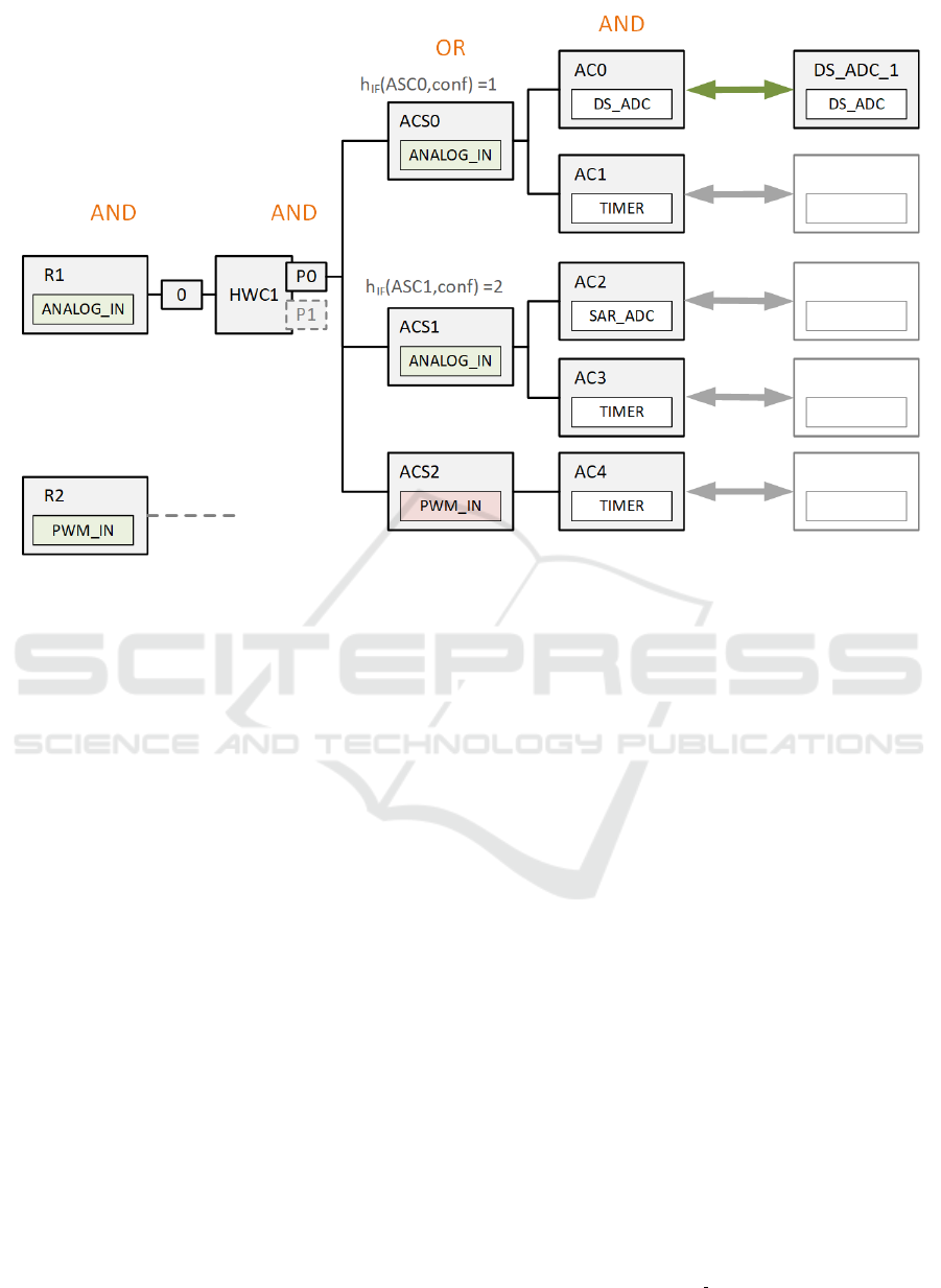
Figure 1: A requirement condition and its possible fulfillments based on a partial configuration.
2.3 Heuristic Search for Optimal
Solutions
Many search algorithms have been presented in the
literature, so it would be prohibitive to review all of
them here. Rather, we focus on the one used in the ex-
periment reported in this paper, A*, a (unidirectional)
search algorithm with certain optimality guarantees.
The traditional best-first search algorithm A*
(Hart et al., 1968) maintains the set OPEN of so-called
open nodes that have been generated but not yet ex-
panded, i.e., the frontier nodes. Much as any best-
first search algorithm, it always selects a node from
OPEN with minimum estimated cost, one of those it
considers “best”. This node is expanded and moved
from OPEN to CLOSED. A* specifically estimates the
cost of some node n with an evaluation function of
the form f (n) = g(n) + h(n), where g(n) is the (sum)
cost of a path found from s to n, and h(n) is a heuris-
tic estimate of the cost of reaching a goal from n, i.e.,
the cost of an optimal path from s to some goal t. If
h(n) never overestimates this cost for all nodes n (it
is said to be admissible) and if a solution exists, then
A* is guaranteed to return an optimal (minimum-cost)
solution (it is also said to be admissible). Under cer-
tain conditions, A* is optimal over admissible unidi-
rectional heuristic search algorithms using the same
information, in the sense that it never expands more
nodes than any of these (Dechter and Pearl, 1985).
3 GOAL CONDITION
A formal specification of goal conditions can be given
in first order logic. As each requirement is speci-
fied as a specific interface type IF(i f ) at a specific
ECU-pin p, we introduce a requirement predicate
REQ(p, IF(i f )).
Each hardware component may support several in-
terface types on its ports. Hence, we introduce a pred-
icate HW (p, IF(i f ), port), which connects an ECU-
pin to the hardware component and the supported in-
terface at a specific port. At each port, there may be a
variety of supported interface types. If a specific inter-
face type is supported, then an assignment constraint
set has to be defined for it, i.e., ACS(port, IF(i f )).
These assignment constraint sets are or-connected:
_
port
i
∈Port
(ACS(port
i
, IF(i f ))) (1)
One assignment constraint set is specified by
and-connected assignment constraints, i.e.,
AC(RType(RT ), SR(R)), where RType denotes
the requested resource type and SR specifies if a
resource has been selected:
ACS(port, IF(i f )) =
^
rt∈REQ RES
i f
AC(RType(RT
rt
), SR(R
rt
))
(2)
Efficiently Finding Optimal Solutions to Easy Problems in Design Space Exploration: A* Tie-breaking
597

A port supports an interface type if there exists at
least one ACS that fulfills its requirements. Hence,
the interface types of all ports of a hardware compo-
nent are defined as:
_
port
i
∈Port
(ACS(port
i
, IF(i f )) (3)
Hence, a specific interface type at a port of a hard-
ware component is defined as:
HW (p, IF(i f ), port) =
_
acs∈port
(ACS
acs
(port, IF(i f ))
(4)
Using these formulas, we can formally specify
that a requirement is fulfilled if a connected hardware
component exists that provides the interface type on a
port:
REQ(p, IF(i f )) = HW (p, IF(i f ), port) (5)
Based on this formula, our goal condition is a
conjunction of all requirements and all ports on con-
nected hardware components for a specific interface
type.
^
i f ∈Req IF
^
p∈HW P
i f
(
_
port
i
∈Port
p
ACS(port
i
, IF(i f ))) (6)
4 ADMISSIBLE HEURISTIC
FUNCTION
For A*, admissibility of the heuristic function is im-
portant for guaranteeing the optimality of solutions
found. For evaluating a configuration in such a func-
tion with respect to its goal achievement, the number
of not (yet) fulfilled conjunctively related goal condi-
tions is counted. In case of disjunctively related con-
ditions, the minimum is taken. The resulting number
can be used as the heuristic value, since each condi-
tion needs at least one application of a transformation
rule. In fact, these can only be activation rules. De-
activation rules may additionally be necessary, in or-
der to deactivate some connection so that another one
needed can be activated at this particular pin. Conse-
quently, this number is less than or equal to the num-
ber of minimal steps to achieve the goal condition,
i.e., this is an admissible heuristic.
This can also be explained more theoretically
based on the meta-heuristic of problem relaxation, see
(Pearl, 1984). A relaxed problem would only need ac-
tivation rules for its solution, i.e., the number calcu-
lated by our heuristic function.
Let us illustrate this in detail using a specific ex-
ample. As already mentioned in the introduction, in
an automotive system like a car, a pedal position sen-
sor is connected to the corresponding ECU. We elab-
orate on the calculation of our heuristic function for
the case of an analogue signal delivered by the sen-
sor. Figure 1 illustrates this example through a re-
quirement condition R1 (at the left) and its possible
fulfillments (in the middle) based on a partial config-
uration (at the right).
The heuristic function optimistically estimates the
distance from a given configuration to a goal by cal-
culating the minimal number of transformation steps
necessary to reach a configuration that fulfills the goal
condition. We explain this using a part of a goal
condition, where the clause of its conjunction corre-
sponding to R1 (as shown in Figure 1) is defined for
this example as
REQ(0, IF(ANALOG IN))
Formally, this means a disjunction of
ACS(P0, IF( )) instantiated for ACS0, ACS1
and ACS2. However, ACS2 has to be discarded,
since its interface type PWM IN is different from the
required ANALOG IN. Of course, only assignment
constraint sets with matching interface types are
taken into account.
The remaining formula can be written as follows,
according to the concrete example shown in Figure 1:
(AC(RType(DS ADC), SR(DS ADC 1))∧
AC(RType(T IMER), SR(Empty)))
∨
(AC(RType(SAR ADC), SR(Empty))∧
AC(RType(T IMER), SR(Empty)))
(7)
SR(DS ADC 1) means that the concrete resource
DS ADC 1 is selected for the assignment constraint
AC0 as shown in the figure. Since the type of the
selected resource matches the required resource type
of the assignment constraint, the predicate AC evalu-
ates to true for this example. Empty as given for the
other assignment constraints in this example means
that no resource is selected (yet) for them. Therefore,
the predicate AC for these examples evaluates to false.
This defines the current partial configuration in the
course of the search that is evaluated heuristically.
For such a partial configuration, the correspond-
ing formula evaluates to false. In order to fulfill the
goal condition, all the remaining and-connected parts
need to evaluate to true as well. This requires certain
transformation steps, and for calculating the admissi-
ble heuristic, we determine the minimum number of
such steps.
ICSOFT 2019 - 14th International Conference on Software Technologies
598

In fact, for making a single AC from false to
true, at least a single transformation step is necessary.
Note, that a single step cannot make more than one
AC true according to the definition of the transforma-
tion rules based on the meta-model.
We define a heuristic function h
IF
of a spe-
cific interface type for a given configuration
(h
IF
(ASCS
IF
,CONF)) in such a way, that it never
over-estimates the minimum number of steps for ful-
filling the requirements of the interface type. Hence,
for or-connected parts, it is necessary to take the min-
imum, so that the heuristic estimate is optimistic. In
the example, therefore, h
IF
(ASC0, con f ) = 1 must be
taken for port P0.
For calculating the complete heuristic function for
a given configuration con f , all requirements and as-
sociated ports must be taken into account. A configu-
ration is specified by all currently selected resources.
Therefore, the heuristic function can be calculated as
follows:
h(con f ) =
∑
r∈Req
∑
p∈Ports(r)
min
acs∈ACS(p,IF(r))
h
IF
(acs, con f )
(8)
5 EXPERIMENT
First, we present our design of the experiment, and
then its results.
5.1 Experiment Design
Since statistical fluctuation was to be expected for dif-
ferent problem instances in the experiment, we de-
fined several ones and included some randomness into
their creation, in order to avoid bias. In addition, we
wanted to systematically get data on the average run-
ning times for different (optimal) solution lengths, in
order to evaluate the effect of scaling with increasing
problem difficulty.
Then we created problem instances with different
solution lengths by generating requirements randomly
(again). This resulted in 75 problem instances for
each solution length, with different starting configura-
tions and different target requirements. From this set,
ten problem instances each were selected randomly
and used for the searches in the experiment. Since we
experienced some variation in the runs of VIATRA2
also regarding the ordering during design space ex-
ploration (i.e., some indeterminism coming from the
tool), which influences the running time depending
on when a solution is found, we ran each problem in-
stance ten times.
The problems created randomly had different dif-
ficulty in terms of reconfigurations required. For sys-
tematically studying the effect of problem difficulty
on the search efficiency, we define two difficulty met-
rics as given in Equations 9 and 10. These metrics
can only be calculated in hindsight, of course, after
both the heuristic value h(s) of the start node s and the
real optimal length C
?
is known, but this is sufficient
for studying the results of various searches. These
metrics do not purely measure the difficult of a given
problem per se, but relative to a given heuristic h and,
of course, the problem difficulty also depends directly
on the optimal solution length C
?
as investigated be-
low. Still, we prefer such measures to the approach of
sorting problem instances according to the effort that
a particular algorithm has to solve them. In the fol-
lowing, we only make use of d
abs
in absolute terms,
since it appears to fit better in our context, but for
other problems, d
rel
in relative terms may be more
appropriate.
d
abs
(s) = C
?
− h(s) (9)
d
rel
(s) =
d
abs
(s)
C∗
(10)
Since our research questions are about search effi-
ciency, we defined dependent variables for measuring
it:
• running time,
• number of states visited.
In order to perform statistical tests, we may con-
sider the null hypothesis that two algorithms to be
compared perform equally well (according to a given
criterion). The resulting p-value gives the probabil-
ity that the data are consistent with the null hypoth-
esis that each method is equally good. Therefore,
only small numbers (below 0.05, for example), indi-
cate that the difference is unlikely to be from chance
fluctuation (the null hypothesis is to be rejected).
We may say that algorithm A “wins” against B
in experiment i when for the corresponding depen-
dent variables a
i
< b
i
holds. For testing the statistical
significance of results about the number of cases in
which one algorithm wins, we consider the null hy-
pothesis that the number of wins is a random event
with probability
1
2
. The sign test is appropriate here,
especially since it requires no specific assumptions
about distributions of the samples. Much as for our
previous search experiments, e.g., in (Kaindl et al.,
1995) for unidirectional search and in (Kaindl and
Kainz, 1997) for bidirectional search, we apply the
sign test for our current experiments as well.
Efficiently Finding Optimal Solutions to Easy Problems in Design Space Exploration: A* Tie-breaking
599
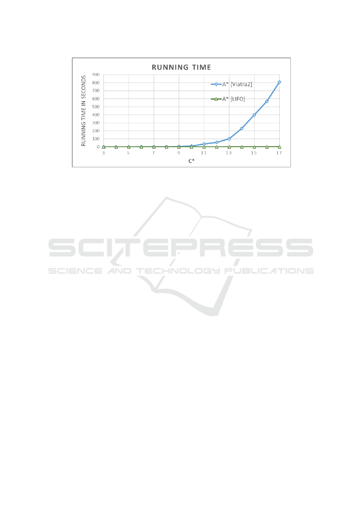
Figure 2: Running times for trivial problems with d
abs
(s) = 0.
We executed the experiment runs on a standard
Windows laptop computer with an Intel Core i7-
8750H Processor (9MB Cache, up to 4.1 GHz, 6
Cores). It has a DDR4-2666MHz memory of 32GB.
The disk does not matter, since all the experimental
data were gathered using the internal memory only.
5.2 Results
On the laptop computer used, we first addressed RQ1
and collected the results of searches with optimal so-
lution lengths (costs) C* for A* with two different
tie-breakers involved, the default one implemented
in VIATRA2, and another one selecting strictly ac-
cording to LIFO from the list of currently minimal f -
values. All the searches found optimal solutions and
guaranteed that they are optimal (in terms of solution
length).
Figure 2 shows the mean running times in
seconds (when no other processes were running
on the laptop computer used) for trivial problems
without any reconfigurations, i.e., d
abs
(s) = 0.
A* [VIATRA2] is the standard implementation in
VIATRA2. It mimics an “arbitrary” selection from
all the ties as indicated in the original definition
of A* by using the PriorityQueue described at
https://docs.oracle.com/javase/10/docs/api/java/util/
PriorityQueue.html. Its scaling behavior is a bit
strange, given that these problems are actually trivial.
A* [LIFO], in contrast, can exploit that fact and
is very efficient on this class of problems. Note,
that A* [FIFO] (using a first-in-first-out strategy
for tie-breaking) is even much worse than A*
[VIATRA2].
Of course, A* [LIFO] (abbreviated in the follow-
ing figures and tables as [LIFO]) cannot have such
an excellent search efficiency with increasing prob-
lem difficulty. This is clearly shown in Figure 3 (with
the broken lines) for d
abs
= 0, 1, 2, and a mix that tries
to model the distribution of problem difficulty in prac-
tice. More precisely, it means that 60 percent would
have d
abs
= 0, 20 percent d
abs
= 1, and 20 percent
d
abs
= 2. d
abs
is abbreviated in all the figures as d.
Generally, the LIFO tie-breaker makes A* also
more efficient than A* [VIATRA2] (the default tie-
breaker in VIATRA2) on more difficult problems, as
indicated by the red square in Figure 3. Hence, we
claim that our experiments provide enough evidence
for answering RQ1 affirmatively. That is, a LIFO
tie-breaker can significantly improve the search effi-
ciency of A* as compared to the default tie-breaker of
the VIATRA2 tool.
For practical purposes, this improvement through
the simple LIFO tie-breaker seemed already sufficient,
and the latest literature (Asai and Fukunaga, 2017)
on tie-breakers for non-zero-cost domains even sug-
gested that it could be the best strategy, anyway. Still,
we found it interesting to investigate on the efficiency
of h-based tie-breakers, which have been heavily used
in the past (see below for this related work). This is
what our RQ2 is all about.
Hence, we also compared A* using LIFO with an-
other tie-breaker that first uses smallest h-values to
break ties (as a primary tie-breaker), and applies a
LIFO tie-breaking policy only as a second-level cri-
terion. Figure 3 also shows a comparison of these tie-
breakers. It indicates that A* [h, LIFO] could be even
more efficient than A* [LIFO] for our problems and
using this heuristic.
This result indicated to answer our RQ2 with no.
However, simply comparing the mean values may have
been misleading, since the results could have come
from chance fluctuation. Hence, as sketched above,
we employed the sign test (using SPSS) for investi-
ICSOFT 2019 - 14th International Conference on Software Technologies
600
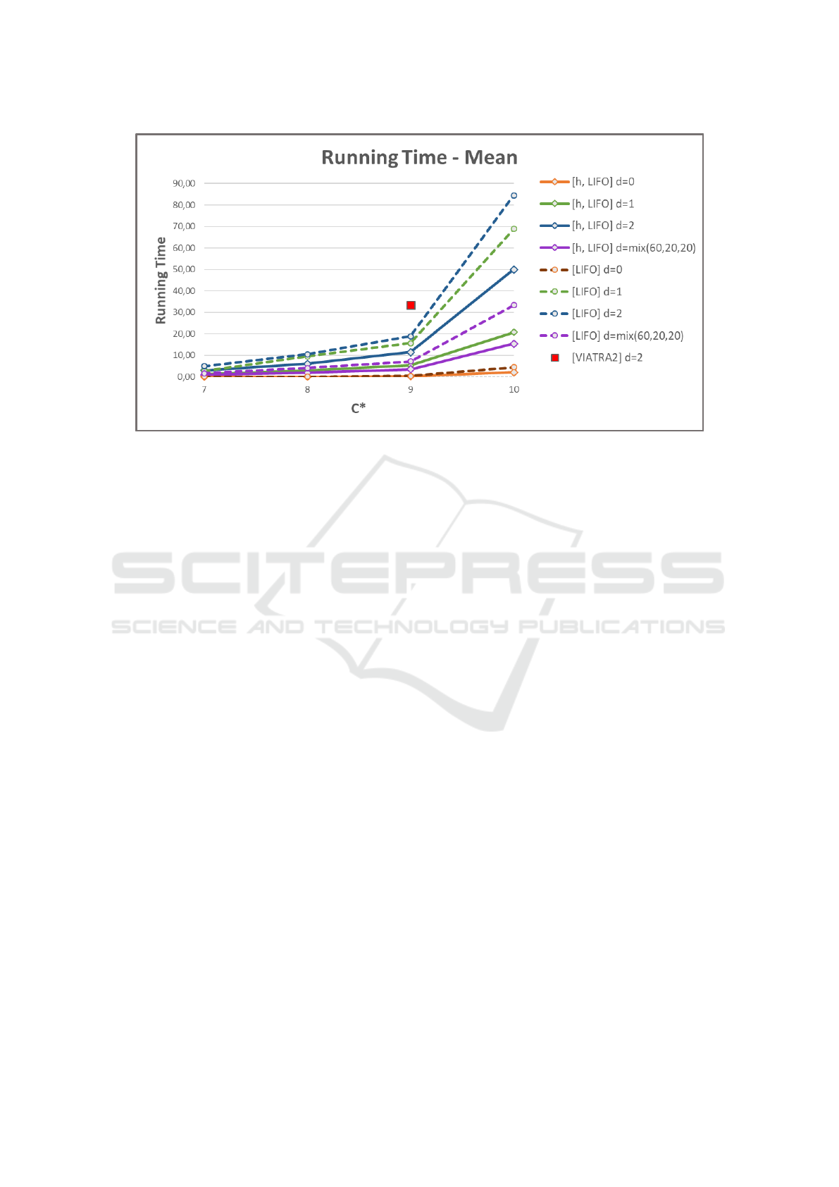
Figure 3: Mean running times of using LIFO as a primary vs. a secondary tie-breaker after minimal h-values on problems
with d
abs
(s) ≥ 0.
gating that. More precisely, we tested the null hy-
pothesis that the median of the differences between
the running times of A* [h, LIFO] and A* [LIFO] is
0, on a significance level of .05. This null hypothe-
sis can be rejected. Therefore, it is unlikely that the
difference comes from chance fluctuation.
Since tie-breaking using h-values did so well here,
the question remained how well it would do with FIFO
or the default VIATRA2 tie-breaker as a secondary
tie-breaker each. The differences between the running
times when using different secondary tie-breakers are
small, as long as the primary h-based tie-breaker is
used. This may be a result of fluctuations regarding
running times on the system or even be influenced by
the used implementations. Hence, we evaluated the
visited states instead to study the relative effective-
ness of the different secondary tie-breakers. Tables 1
and 2 show the mean and median data, respectively.
Still, these numbers are close, and the question
remains whether any of these secondary tie-breakers
makes a real difference when the primary tie-breaker
is based on the h-values. Since the results could have
come from chance fluctuation, we employed the sign
test again for investigating that. More precisely, we
tested a null hypothesis for each problem difficulty:
the median of the pair-wise differences between the
visited states of A* [h, LIFO], A* [h, VIATRA2] and
A* [h, FIFO] is 0, on a significance level of .05, for
d
abs
(s) = 0, 1, 2. Since these null hypotheses cannot
be rejected, it seems as though secondary tie-breakers
do not really matter in our domain when the primary
tie-breaker is based on the h-values.
Overall, it seems clear that the answer to our RQ2
is no. That is, a LIFO tie-breaker is not generally bet-
ter in terms of A* search efficiency than a tie-breaker
using minimal heuristic values, as the recent results
in the literature suggest for non-zero-cost domains,
see (Asai and Fukunaga, 2017). At least in our do-
main and for unit-costs, it is most likely even worse.
6 RELATED WORK ON A*
TIE-BREAKING
Recently, there was increasing interest in tie-breaking
strategies for A*, but primarily for zero-cost domains.
(Asai and Fukunaga, 2016) discussed tie-breaking
strategies for zero-cost actions and showed that a
custom tie-breaking strategy can have significant im-
pact on the search algorithm performance. (Asai and
Fukunaga, 2017) expanded on their previous results
and introduced two new classes of tie-breaking strate-
gies. They demonstrated that their approach signif-
icantly outperformed standard strategies on domains
with zero-cost actions. (Corrła et al., 2018) proposed
a tie-breaking strategy using cost adaptation that guar-
antees optimal expansion for zero-cost domains. In
contrast, our problems have unit costs for transforma-
tion steps (greater than zero), where these new ap-
proaches for zero-cost domains are not applicable.
For non-zero-cost domains, such as ours with unit-
costs, which A* was originally defined for, there was
for a long time some rumor on how to tie-break most
effectively, but there were no really founded general
results. (Helmert, 2006) used a FIFO tie-breaking
Efficiently Finding Optimal Solutions to Easy Problems in Design Space Exploration: A* Tie-breaking
601

Table 1: Mean numbers of visited states of A* searches using different tie-breaking strategies on problems with different
d
abs
(s).
[h, LIFO] [h, VIATRA2] [h, FIFO]
C* 0 1 2 0 1 2 0 1 2
7 131 2,676 6,043 210 2,603 6,024 177 2,665 6,156
8 110 7,001 12,159 107 7,138 12,065 120 7,058 12,132
9 603 12,267 22,968 947 12,668 22,529 854 12,640 22,918
10 4,526 46,506 95,242 2,911 47,084 95,625 4,528 47,209 94,927
Table 2: Median numbers of visited states of A* searches using different tie-breaking strategies on problems with different
d
abs
(s).
[h, LIFO] [h, VIATRA2] [h, FIFO]
C* 0 1 2 0 1 2 0 1 2
7 89 2,531 6,349 90 2,565 6,259 92 2,640 6,539
8 107 7,440 14,157 99 7,346 13,834 108 7,435 14,121
9 131 11,276 26,670 129 12,351 27,022 128 12,411 25,962
10 150 48,175 88,406 152 50,016 87,816 147 47,108 87,227
strategy in his A*-based planner named Fast Down-
ward. In contrast, (Hansen and Zhou, 2007) stated
that “It is well-known that A* achieves best perfor-
mance when it breaks ties in favor of nodes with least
h-cost”. (Holte, 2010) stated that “A* breaks ties in
favor of larger g-values, as is most often done”, and
this is equivalent to tie-breaking according to smallest
h-values. (R
¨
oger and Helmert, 2010) also used small-
est h-values to break ties, and applied for still remain-
ing ties a FIFO tie-breaking policy as a second-level
criterion. Also (Burns et al., 2013) used smallest h-
values to break ties, but applied a LIFO tie-breaking
policy (instead of FIFO) as a second-level criterion.
Recently, (Asai and Fukunaga, 2017) reported
on experiments using the IPC Planning Competition
Benchmarks and concluded that breaking ties using
smallest h-values is not necessarily the best strat-
egy in such non-zero-cost domains, while simply us-
ing LIFO may even be better. This also depends,
however, on the second-level criterion used after tie-
breaking using smallest h-values. Their experiments
measured the number of problems solvable with given
resources, while our experiments compared node ex-
pansions and running times on problems that all the
compared variants solved (in the HSI domain). We
also investigated statistical significance of the key re-
sults.
7 DISCUSSION
Interestingly, our results in our real-world domain as
shown above are more conformant to previous rumor
than to the results of (Asai and Fukunaga, 2017). Af-
ter all, our data indicate a statistically significant su-
periority of using minimal h-values as a tie-breaker
(independently of using LIFO or FIFO as a secondary
tie-breaker) over directly using LIFO as a tie-breaker.
This is in contrast to Asai and Fukunaga’s statement
based on their experiments using IPC domains (Asai
and Fukunaga, 2017, p. 69):
“Tie-breaking according to the heuristic value
h, which is frequently mentioned in the heuris-
tic search literature, has little impact on the
performance as long as lifo default criterion
is used — in other words, a lifo tie-breaking
policy is sufficient for most IPC domains.”
The fact that using minimal h-values was better
than LIFO as a tie-breaker in our experiments may be
the result of several contributing factors. First, our
problems have unit costs, and transformation steps
are only included into the search if they contribute to
achieving the given goal condition. Thus, while each
step costs one unit, it also gets one step closer to a goal
state, which reduces the h-value by one. Therefore,
the resulting nodes from this node expansion have
ICSOFT 2019 - 14th International Conference on Software Technologies
602

now the smallest h-value for the h-based tie-breaker.
Given that, secondary tie-breakers such as LIFO or
FIFO do not have much influence on the search per-
formance. In contrast, LIFO as a tie-breaker (without
consideration of h-values) implements a strict depth-
first search among the nodes with the same f -values,
and it may not always lead to an optimal path towards
a goal node when starting it from a node with a greater
than minimal h-value. This is especially the case with
d
abs
> 0, where reconfiguration is necessary.
8 CONCLUSION
Some real-world domains appear to have special
kinds of problems. In the case of HSIs, they show
a mix of trivial problems (without an actual need
for search) with problems including reconfiguration
(which require search for finding optimal solutions).
While previous theoretical work indicated the need
for a tie-breaker of A* instead of random selection
from several nodes with the minimum value, we are
not aware of such dramatic differences that we have
observed through using different tie-breakers. They
appear to be due to the problems having unit costs
and that they are often — but not always — easy.
Summarizing, the contributions of this paper are
• A more theoretical treatment of defining an ad-
missible heuristic in this HSI domain,
• A dramatic improvement over such HSI searches
with the default implementation of A* in the
VIATRA2 tool, especially for trivial problems,
• Definitions of metrics for measuring the difficulty
of problems,
• Analysis of statistical significance for the cases
with relatively close results from different tie-
breakers, and
• New results and insights on tie-breaking using
minimum h-values vs. LIFO in a real-world do-
main with unit-costs.
Based on our results on h-based tie-breaking vs.
the recent results on LIFO-based tiebreaking by (Asai
and Fukunaga, 2017), and considering the diversity
of statements in the previous related work about such
tie-breakers, we conjecture that there is no generally
best tie-breaker for A* in non-zero-cost domains. It
seems as though this is domain-specific, and future
work should find out the criteria for the preference of
one such tie-breaker over others.
ACKNOWLEDGEMENTS
We would like to thank Oszkar Semerath from the
VIATRA team for having pointed us to the place
in the implementation where the tie-breaker can be
changed.
The InteReUse project (No. 855399) is funded
by the Austrian Federal Ministry of Transport, In-
novation and Technology (BMVIT) under the pro-
gram “ICT of the Future” between September 2016
and August 2019. More information can be found at
https://iktderzukunft.at/en/.
REFERENCES
Asai, M. and Fukunaga, A. (2017). Tie-Breaking Strategies
for Cost-Optimal Best First Search. J. Artif. Intell.
Res., 58:67–121.
Asai, M. and Fukunaga, A. S. (2016). Tiebreaking Strate-
gies for A* Search: How to Explore the Final Fron-
tier. In Schuurmans, D. and Wellman, M. P., editors,
Proceedings of the Thirtieth AAAI Conference on Ar-
tificial Intelligence, February 12-17, 2016, Phoenix,
Arizona, USA., pages 673–679. AAAI Press.
Bergmann, G., D
´
avid, I., Heged
¨
us,
´
A., Horv
´
ath,
´
A., R
´
ath, I.,
Ujhelyi, Z., and Varr
´
o, D. (2015). Viatra 3: A Reactive
Model Transformation Platform. In Kolovos, D. and
Wimmer, M., editors, Theory and Practice of Model
Transformations, pages 101–110, Cham. Springer In-
ternational Publishing.
Burns, E., Ruml, W., and Do, M. B. (2013). Heuris-
tic Search when Time Matters. J. Artif. Int. Res.,
47(1):697–740.
Corrła, A. B., Pereira, A. G., and Ritt, M. (2018). Analyz-
ing Tie-Breaking Strategies for the A* Algorithm. In
Proceedings of the Twenty-Seventh International Joint
Conference on Artificial Intelligence, IJCAI-18, pages
4715–4721. International Joint Conferences on Artifi-
cial Intelligence Organization.
Dechter, R. and Pearl, J. (1985). Generalized best-
first strategies and the optimality of A
∗
. J. ACM,
32(3):505–536.
Hansen, E. A. and Zhou, R. (2007). Anytime Heuristic
Search. J. Artif. Int. Res., 28(1):267–297.
Hart, P., Nilsson, N., and Raphael, B. (1968). A formal
basis for the heuristic determination of minimum cost
paths. IEEE Transactions on Systems Science and Cy-
bernetics (SSC), SSC-4(2):100–107.
Helmert, M. (2006). The Fast Downward Planning System.
J. Artif. Int. Res., 26(1):191–246.
Holte, R. C. (2010). Common Misconceptions Concerning
Heuristic Search. In Felner, A. and Sturtevant, N. R.,
editors, Proceedings of the Third Annual Symposium
on Combinatorial Search, SOCS 2010, Stone Moun-
tain, Atlanta, Georgia, USA, July 8-10, 2010. AAAI
Press.
Efficiently Finding Optimal Solutions to Easy Problems in Design Space Exploration: A* Tie-breaking
603

Kaindl, H. and Kainz, G. (1997). Bidirectional heuristic
search reconsidered. Journal of Artificial Intelligence
Research (JAIR), 7:283–317.
Kaindl, H., Kainz, G., Leeb, A., and Smetana, H. (1995).
How to use limited memory in heuristic search. In
Proc. Fourteenth International Joint Conference on
Artificial Intelligence (IJCAI-95), pages 236–242. San
Francisco, CA: Morgan Kaufmann Publishers.
Pearl, J. (1984). Heuristics: Intelligent Search Strate-
gies for Computer Problem Solving. Addison-Wesley,
Reading, MA.
Rathfux, T., Kaindl, H., Hoch, R., and Lukasch, F. (2019).
An Experimental Evaluation of Design Space Explo-
ration of Hardware/Software Interfaces. In Damiani,
E., Spanoudakis, G., and Maciaszek, L. A., editors,
Proceedings of the 14th International Conference on
Evaluation of Novel Approaches to Software Engi-
neering, ENASE 2019, Heraklion, Crete, Greece, May
4-5, 2019., pages 289–296. SciTePress.
R
¨
oger, G. and Helmert, M. (2010). The More, the Mer-
rier: Combining Heuristic Estimators for Satisficing
Planning. In Brafman, R. I., Geffner, H., Hoffmann,
J., and Kautz, H. A., editors, Proceedings of the 20th
International Conference on Automated Planning and
Scheduling, ICAPS 2010, Toronto, Ontario, Canada,
May 12-16, 2010, pages 246–249. AAAI.
ICSOFT 2019 - 14th International Conference on Software Technologies
604
