Trading Memory versus Workload Overhead in Graph Pattern Matching

on Multiprocessor Systems

Alexander Krause

1 a

, Frank Ebner

2 b

, Dirk Habich

1 c

and Wolfgang Lehner

1 d

Technische Universit

at Dresden, Database Systems Group, Dresden, Germany

University of Applied Sciences W

urzburg-Schweinfurt, Faculty of Computer Science and Business Information Systems,

urzburg, Germany

Keywords:

Graph Processing, In-memory, Bloom Filter, Multiprocessor System, NUMA.

Abstract:

Graph pattern matching (GPM) is a core primitive in graph analysis with many applications. Efﬁcient process-

ing of GPM on modern NUMA systems poses several challenges, such as an intelligent storage of the graph

itself or keeping track of vertex locality information. During query processing, intermediate results need to

be communicated, but target partitions are not always directly identiﬁable, which requires all workers to scan

for requested vertices. To optimize this performance bottleneck, we introduce a Bloom ﬁlter based workload

reduction approach and discuss the beneﬁts and drawbacks of different implementations. Furthermore, we

show the trade-offs between invested memory and performance gain, compared to fully redundant storage.

1 INTRODUCTION

To satisfy the ever-growing computing power de-

mand, hardware vendors improve their single hard-

ware systems by providing an increasingly high de-

gree of parallelism. In this direction, large-scale sym-

metric multiprocessor (SMP) are the next parallel

hardware wave (Borkar et al., 2011). These SMP sys-

tems are characterized by each processor having the

same architecture e.g. a multicore and all multipro-

cessors share a common memory space. This SMP

type can be further classiﬁed into SMP with uniform

memory access (UMA) and SMP with non-uniform

memory access (NUMA), with the latter being the

dominant approach. Both allow all processors to ac-

cess the complete memory, but with different connec-

tivity. This is a completely different hardware ap-

proach, since former processor generations got more

performant by increasing their core frequency, lead-

ing to a higher performance at a free lunch. This effect

came to an end due to power and thermal constraints.

Thus, speedups will only be achieved by adding more

parallel units. However, these have to be utilized in an

appropriate way (Borkar et al., 2011; Sutter, 2005).

In addition to a very high number of cores, these

large-scale NUMA-SMP systems also feature main

https://orcid.org/0000-0002-2616-8739

https://orcid.org/0000-0002-4698-8232

https://orcid.org/0000-0002-8671-5466

https://orcid.org/0000-0001-8107-2775

memory capacities of several terabytes (Borkar et al.,

2011; Kissinger et al., 2014). For applications like

graph processing, this means that large graphs can

be stored completely in memory and efﬁciently pro-

cessed in parallel. Fundamentally, the meaning of

graphs as data structure is increasing in a wide and

heterogeneous spectrum of domains, ranging from

recommendations in social media platforms to ana-

lyzing protein interactions in bioinformatics (Paradies

and Voigt, 2017). Based on that, graph analytics is

also increasingly attractive to acquire new insights

from graph-shaped data. In this context, graph pat-

tern matching (GPM) is an important, declarative,

topology-based query mechanism and a core primi-

tive. The pattern matching problem is to ﬁnd all pos-

sible subgraphs within a graph that match a given pat-

tern. The calculation of graph patterns can get pro-

hibitively expensive due to the combinatorial nature.

To efﬁciently compute graph patterns on such large-

scale systems, we already proposed a NUMA-aware

GPM infrastructure in (Krause et al., 2017a; Krause

et al., 2017b), which is based on a data-oriented ar-

chitecture (DORA) (Kissinger et al., 2014; Pandis

et al., 2010). As Figure 1 shows, our infrastructure

is characterized by implicitly partitioning graphs into

small partitions and each partition is placed in the lo-

cal memory of a speciﬁc NUMA node. Moreover,

we use a thread-to-data mapping, such that each local

hardware thread runs a worker. These are limited to

operate exclusively on local graph partitions. Based

on that, the calculation of pattern matching ﬂows from

400

Krause, A., Ebner, F., Habich, D. and Lehner, W.

Trading Memory versus Workload Overhead in Graph Pattern Matching on Multiprocessor Systems.

DOI: 10.5220/0008116904000407

In Proceedings of the 8th International Conference on Data Science, Technology and Applications (DATA 2019), pages 400-407

ISBN: 978-989-758-377-3

Figure 1: Data-oriented graph partitioning with thread as-

signment.

thread to thread depending on the data being accessed.

Our previous work shows good scalability, whereby

the graph partitioning has a high performance impact.

This is remedied by a set of indicators, which we use

to select the optimal partitioning strategy for a given

graph and workload in (Krause et al., 2017a).

Our Contribution. DORA enables us to fully uti-

lize all cores to efﬁciently process a pattern query in

a highly parallel way. However, since we need to ex-

plicitly exchange intermediate results between work-

ers, our whole approach depends on how we store

the graph. If we only consider outgoing edges in a

directed graph, we cannot always determine exactly

to which partition (workers) the intermediate results

have to be sent for further processing. In this case,

we have to send them to all workers using a broad-

cast. This can be mitigated by also storing incom-

ing edges as full redundancy. The consequence is

doubled memory consumption, but we can send uni-

casts, because target vertices can be directly looked

up. We propose to employ a Bloom ﬁlter based solu-

tion, which reduces broadcasts to a couple of unicasts,

while only requiring a fraction of the memory over-

head compared to full redundancy. Thus, our trade off

for memory vs. workload overhead remains bearable.

Outline. This paper is structured as follows: In

section 2, we brieﬂy introduce our graph data model

including an illustration of GPM. Then, we introduce

our Bloom ﬁlter-based approach to efﬁciently trade

memory versus workload overhead for GPM on large-

scale NUMA-SMP systems in Section 3. Based on

that, Section 4 describes selected evaluation results.

Finally, we close the paper with related work and a

short conclusion in Sections 5 and 6.

2 DATA MODEL AND PATTERN

MATCHING

Within this paper, we focus on edge-labeled multi-

graphs (ELMGs) as a general and widely employed

graph data model (Pandit et al., 2007; Otte and

Rousseau, 2002). An ELMGs G(V,E, ρ, Σ, λ) con-

sists of a set of vertices V, a set of edges E, an inci-

dence function ρ : E → V ×V , and a labeling function

λ : E → Σ that assigns a label to each edge. Hence,

ELMGs allow any number of labeled edges between

a pair of vertices, with RDF being a prominent exam-

ple (Decker et al., 2000). This model does not im-

pose any limitation, since e.g. property graphs can

also be expressed as directed ELMGs through intro-

ducing additional vertices and edges for properties.

Storing a graph can be done manifold. One of

the most intuitive and straightforward ways is to store

all outgoing edges of a vertex as an edge list, which

we call outgoing edge storage (OES). This way, the

topology of the graph can be represented precisely

and lossless. To conform with DORA, we store all

outgoing edges of one vertex within the same parti-

tion. Measures for balanced partitioning are neces-

sary and applied, but out of scope of this work.

As mentioned in Section 1, GPM is a declara-

tive topology-based querying mechanism. The query

is given as a graph-shaped pattern and the result is

a set of matching subgraphs (Tran et al., 2009). A

well-studied mechanism for expressing such query

patterns are conjunctive queries (CQs) (Wood, 2012),

which decompose the pattern into a set of edge pred-

icates each consisting of a pair of vertices and an

edge label. Following this, the example query (A) →

(RedVertex) → (B) is decomposed into the conjunc-

tive query {(V

) → (V

red

), (V

red

) → (V

)}. Answer-

ing this query is easy using OES for Figure 1, since

we only need to lookup all matches for V

ﬁrst and

do the same for all found (V

red

) subsequently. This

is done by sending a single unicast message between

two workers, communicating the intermediate results.

This is straightforward, since the OES is partitioned

by the vertex ids, which can be directly looked up to

ﬁnd their corresponding partition. Adding edge labels

speeds up this process, as they increase the queries se-

lectivity. However, reversing one of the edges, e.g. as

in (A) → (RedVertex) ← (B), the process gets com-

plicated. The ﬁrst step remains the same, but ﬁnding

all vertices (V

) now requires a broadcast message

targeting all partitions. The OES does not allow di-

rect lookup of target vertices, thus we need to activate

all workers to scan their partitions, if there is a (V

which has (V

red

) as target vertex. Hence, the work-

ers processing the grey and yellow partition perform

unnecessary work which should be avoided.

Trading Memory versus Workload Overhead in Graph Pattern Matching on Multiprocessor Systems

401

3 TRADING MEMORY VERSUS

WORKLOAD OVERHEAD

Processing GPM on NUMA-SMP systems poses sev-

eral challenges. With the data partitioning being a

prominent example, another obstacle is the available

vertex locality information, based on the edge stor-

age. In our previous work (Krause et al., 2017b),

we have shown the inﬂuence of incomplete vertex lo-

cality information, due to OES. We found, that an-

swering queries with backward edges results in the

activation of all workers (i.e. sending a broadcast),

to ﬁnd out, which partition actually contains the re-

quested vertices.The resulting workload overhead can

have signiﬁcant performance impact and should thus

be avoided; i.e. the reduction of messages in the sys-

tem is highly desirable. A straightforward solution

for this problem is to simply store full redundancy,

i.e. reversing all edges and store them partitioned by

the target vertex as incoming edges. This incoming

edge storage (IES) adds a twofold storage overhead,

but can increase the system performance dramatically.

That is, since workers, which do not contain a re-

quested vertex from a broadcast, do not get stalled

with excess calls and can perform their actual work in

time. However, when the stored graph grows or when

there is a tighter memory budget, this approach is not

feasible anymore. The consequence is to ﬁnd a trade

off between the invested memory for the gained per-

formance. There is one direct ﬁt for this requirement:

A Bloom ﬁlter. The probabilistic data structure can

be scaled in its size, which implicates varying accu-

racy and thus allows us to trade invested memory for

workload.

Bloom Filter Design Aspects. Instead of storing

each element completely and as-is, requiring large

amounts of storage capacity, the Bloom ﬁlter refers

to a few bits to remember a vertex’ presence. Filling

is performed by a hash function, which is applied to

the vertex id, with the result denoting the slot number

into a bitﬁeld, denoting the bit to set to 1. To check

whether a vertex id is present, its hash is calculated

and the bitﬁeld is checked, whether it contains a 1 or 0

at the index given by the hash. By not fully describing

each vertex, this represents a probabilistic data struc-

ture with a false positive rate, i.e. returning true, even

if a vertex is not present. Yset, false negatives, i.e. re-

turning a false for a vertex which is actually present,

are forbidden. Due to collisions, using just one bit

per vertex, usually yields false positive rates above

an acceptable level. Hence implementations use more

than one hash per element, where H

(x)6=

(x) ∀x

and i 6= j. For each hash, a 1 is stored within the cor-

responding bit. When querying, the element might

exist, if all bitﬁeld indices contain a 1. The false pos-

itive rate p thus depends on the number K of hashes

used per vertex, and the number of bits M within the

bitﬁeld. The approximate number of bits required for

storing N vertices at a desired false positive rate, is

given by (Bloom, 1970; Broder and Mitzenmacher,

2003), cf. (1). This yields a space requirement of

≈10 bits per vertex for a false positive rate of 1 %,

which is much less compared to fully redundant stor-

age. Similar rules hold true for the optimal number

of hashes, (Broder and Mitzenmacher, 2003), see (2).

With the number of stored bits being dynamic, we can

adjust the Bloom ﬁlter size to yield a reasonable false

positive rate.

M ≈ −1.44N log

(p) . (1)

K =

ln2 ≈ −1.44 ln(2)log

(p) . (2)

The computational cost of the Bloom ﬁlter mainly de-

pends on the performance of the hash algorithms, con-

verting arbitrary data into a numeric value, uniformly

throughout the whole range, that is, the size of the bit-

ﬁeld. While 64 bit unsigned integer vertex ids already

are numeric values, ids can not be used as-are, since

the bitﬁeld will be much smaller than 2

bits. Yet, a

hash function for this kind of input data is much sim-

pler, as it just needs to distribute all potential vertex

ids uniformly among the available bitﬁeld slots. This

is commonly achieved by multiplying the id x with

some number a

, limiting the result to the number of

slots using the modulo operator:

(x) = y = a

· x (mod M), x ∈ N, a

∈ N

. (3)

However, this operator is known to be very costly

(Granlund, 2017). Thus we exploit the residue class

ring property (4). For 64 bit unsigned integer ver-

tex ids, which are of base 2, the last k digits of (x)

are given by applying a bitmask, or bitwise and, of

− 1) to (x)

. Following this approach, we can

alter (3) by replacing the modulo operator with bit-

wise and while selecting prime numbers for a

, since

they yield best uniformity results (Hull and Dobell,

1962). Therefore, we limit our Bloom ﬁlter sizes to

, k ∈ N and use (5) as our hash algorithm, which we

call PrimeHash henceforth.

(x)

base

(mod base

) = last k digits of (x)

base

. (4)

(x) = y = (a

· x) ∧ (M − 1) . (5)

Besides returning false positives, Bloom ﬁlters suf-

fers from additional drawbacks that need to be con-

sidered: As only single bits are stored, collisions can

not be tracked, and vertices can not be deleted from

the ﬁlter. For dynamic graphs, where many deletions

occur, the false positive rate might reach unacceptable

DATA 2019 - 8th International Conference on Data Science, Technology and Applications

402

levels over time. To overcome collisions ambiguities,

the counting Bloom ﬁlter stores the number of ele-

ments contributing to each slot. This enables deletion

by decreasing the corresponding number, but requires

additional memory to store counters instead of bits.

Similar to the missing support for deletion, is the lack

of runtime scalability. The more vertices are added to

the ﬁlter, the more bits are set to 1. Eventually, all bits

will be set and the ﬁlter is useless. As the Bloom ﬁl-

ter does not store the vertices themselves, growing is

not supported by the data structure on its own, but re-

quires re-scanning the whole graph, rehashing all ver-

tices. To reach an acceptable false positive rate for a

given graph, the Bloom ﬁlters size, and thus the num-

ber of to-be-added vertices, must be known before-

hand. Scalable Bloom ﬁlters can mitigate this issue,

but within this paper we concentrate on static graphs

and static Bloom ﬁlters, to reduce complexity. This

does not limit the applicability of our approach, since

static and dynamic graphs share the same messaging

procedure, and processing GPM on dynamic graphs

would equally beneﬁt from our optimization. A scal-

able Bloom ﬁlter with a dynamic graph would only

add to computational complexity, but not to the mes-

saging issue, and is thus ignored.

4 EVALUATION

Our developed GPM engine is a research prototype,

which builds upon the DORA, targeting NUMA-SMP

systems as mentioned in Section 1. We have tested

our GPM engine against three different graphs. One

is a bibliographical network, the second represents a

social network and the third graph stands for a protein

network, where the three are called biblio, social and

uniprot respectively henceforth. All three graphs are

generated with gMark (Bagan et al., 2017) to consist

of approx. 1 M edges each. For our experiments, we

store the graphs both with OES and fully redundant

(OES+IES), as described in Sections 2 and 3. Our

evaluation hardware consists of a four socket NUMA

system, each equipped with an Intel(R) Xeon(R) Gold

6130 CPU @ 2.10GHz, resulting in 128 hardware

threads with a total of 384 GB of main memory. With

this system, we want to examine the messaging be-

havior between a large number of workers, even if its

main memory is a bit over-provisioned for the gen-

erated datasets. This section is structured as follows:

First, we want to emphasize the necessity of a care-

ful Bloom ﬁlter design. Second, we show the beneﬁts

and drawbacks of both fully redundant storage versus

the Bloom ﬁlter optimized storage. Third, we conduct

extensive experiments and run the example queries

against the aforementioned storage settings, with and

without an additionally applied Bloom ﬁlter in differ-

ent parts of our GPM engine. To underline the impor-

tance of an appropriate Bloom ﬁlter design, we show

its read/write performance in Figure 2. Figure 2(a)

shows the write results for our testing machine. As

can be seen, the counting ﬁlter from Section 3 yields

the same insertion performance as storing only one bit

in a larger type, since their points almost overlap for

32 bit or 64 bit data types. Using packed data storage,

where each hashed bit is stored using an actual bit

within a larger scalar value, proves to be the fastest

storage solution. This is most likely due to reduced

storage requirements, ﬁtting the internal caches of the

CPU. Figure 2(b) proves the superiority of our bitwise

and based PrimeHash against the traditional modulo

operator. In terms of fairness, we ran our experi-

ments for the modulo operator against Bloom ﬁlters

using the same size as required for PrimeHash (2

see Eq. (4)) as well as the exactly calculated size ac-

cording to Eq. 1. The ﬁgure shows, that using bitwise

and clearly outperforms the modulo variants within

both scenarios: always calculating all hash functions

according to Eq. (2), or returning after the ﬁrst false

(early-out).

For our graph related experiments, we have used

the partitioning strategies as explained in (Krause

et al., 2017a). From that paper, we have chosen

HashVertices, RoundRobinVertices and Multilevel k-

Way partitioning. In summary, the ﬁrst two parti-

tion the graph following their names and the k-Way

partitioning is a sophisticated graph partitioning al-

gorithm, which ﬁrst partitions the graph very coarse

grained but later reﬁnes the result in subsequent steps.

In this paper, we use the METIS 5.1 implementation

of that algorithm (Karypis and Kumar, 1998). Fur-

thermore, we have chosen two different graph pat-

terns for our analysis. The query Q1 forms a rectan-

gle consisting of four vertices and four edges and the

query Q2 represents a V shaped pattern consisting of

ﬁve vertices and four edges. Both queries have a dif-

ferent amount of backward edges at signiﬁcant eval-

uation steps to emphasize their impact. This leads to

diverse communicational behavior, which allows us

to show the effect of both full redundancy and Bloom

ﬁlter usage standalone and in combination.

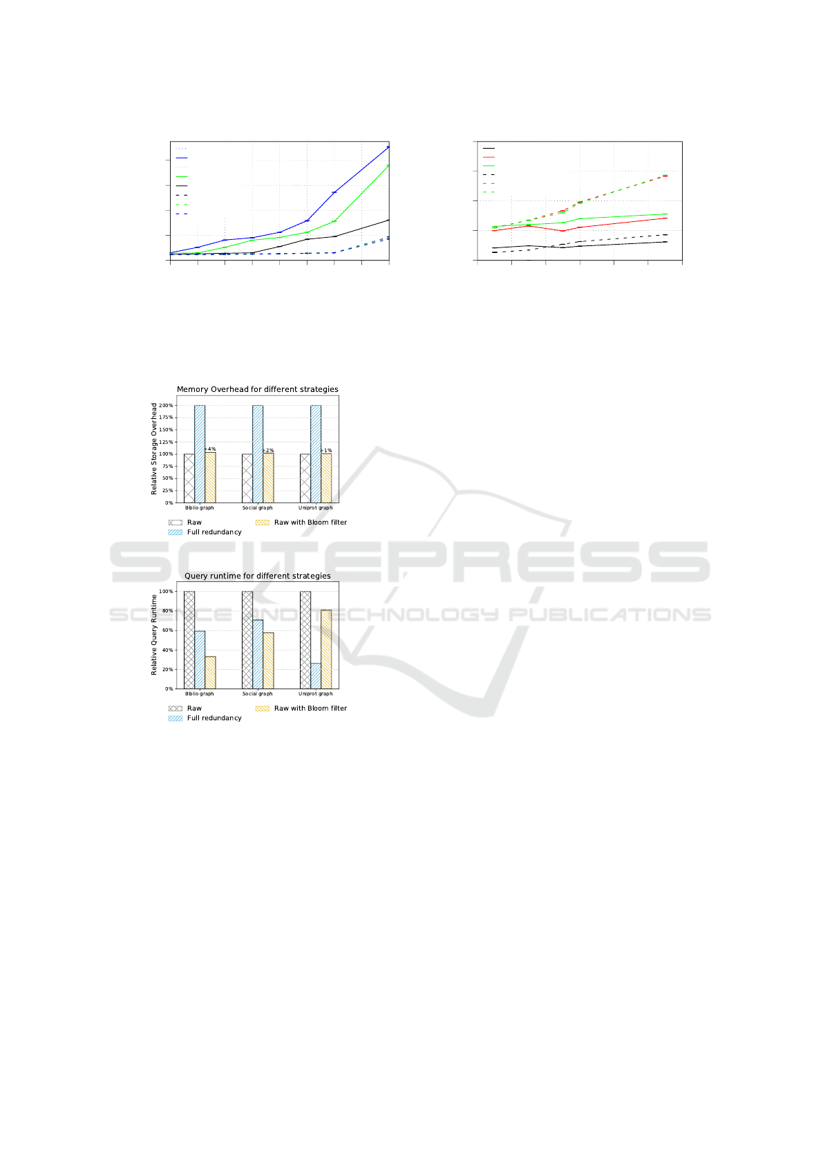
Figure 3(a) depicts the general memory invest-

ment for the previously mentioned improvements.

The ﬁgure shows the relative storage overhead for full

redundancy, which is obviously always twice as much

as OES, compared to the standard storage. Adding a

Bloom ﬁlter to the raw storage does not add much

in terms of memory needed, however its performance

gain can be remarkable. Figure 3(b) shows the result-

Trading Memory versus Workload Overhead in Graph Pattern Matching on Multiprocessor Systems

403

time [ms]

BitSet size [number of bits]

Counting 64

Single 64

Counting 32

Single 32

Single 8

Packed 8

Packed 32

Packed 64

(a) Insert 5 million entries.

0.5

1.5

4 6 8 10 12 14 16

time [s]

Bits per item [number of bits]

BF AND (e-out)

BF MOD1 (e-out)

BF MOD2 (e-out)

BF AND (all)

BF MOD1 (all)

BF MOD2 (all)

(b) Query 1 million items.

Figure 2: Time to perform different actions, based on the Bloom ﬁlter storage strategy (left) and comparing bitwise and [BF

AND] vs. the modulo operator [BF MOD1/2] (right). While [BF MOD1] uses the size required by Eq. (4), [BF MOD2] refers

to the size from Eq. (1) instead.

(a) Relative storage overhead.

(b) Relative query performance for Q1.

Figure 3: Invested memory vs. gained performance for full

redundancy against a Bloom ﬁlter within the data partitions,

M = 2

, k-Way partitioning.

ing query run times for all storage strategies. The raw

storage is only the slowest and adding redundancy or a

Bloom ﬁtler increases the performance. Interestingly,

for the Biblio use case, the Bloom ﬁlter outperforms

even the redundant storage. The reason is, that the

Bloom ﬁlter can sort out edge requests for target ver-

tices, that are not stored in the partition, which is not

covered by redundant storage.

When implementing the Bloom ﬁlter, we can do

that on multiple locations. Obvious candidates are the

data partitions themselves, which makes the Bloom

ﬁlter behave more like a secondary index. By doing

this, the system still needs to activate all workers to

ﬁnd out, if a partition contains a requested vertex. On

the other hand, we still exploit all cores to perform

the ﬁltering process in parallel. A second possibility

is to place the Bloom ﬁlter together with the partition-

ing information. This allows us to directly check, if a

certain partition possibly contains a requested vertex.

The routing based workload reduction can give an-

other performance increase as shown in Figure 4(a),

since workers are not unnecessarily activated. How-

ever, looking up target partitions is an inherently se-

rial code segment. Thus, iterating over all partition re-

lated Bloom ﬁlters leads to increased local overhead,

which linearly increases with the amount of partitions

in the system.

Besides varying the Bloom ﬁlter location, we can

also swap the underlying partitioning. Figure 4(b)

depicts the relative query runtime for routing based

workload optimization using the RoundRobinVertices

(RRV) partitioning strategy. We observe completely

different query performance for both the redundant

and Bloom ﬁlter supported query execution. In addi-

tion, neither the RRV nor the k-Way partitioning strat-

egy yield globally optimal results, which supports our

ﬁndings from previous work (Krause et al., 2017a).

Yet, the Bloom ﬁlter approach increases the query

performance for both underlying partitionings.

After showing the performance gain for Q1, we

now discuss selected results for Q2 in Figure 4. As

for Q1, we achieve a performance gain with both the

redundant storage as well as the Bloom ﬁlter employ-

ment. However, here we see a signiﬁcant difference

between the two, at least for the Uniprot graph. We

identiﬁed, that an extraordinarily high amount of in-

termediate results occurs right before evaluating the

backward edge and thus, the aforementioned serial

checking of Bloom ﬁlter becomes a bottleneck.

Based on these observations, we can state that em-

DATA 2019 - 8th International Conference on Data Science, Technology and Applications

404

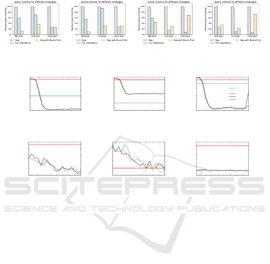
(a) Q1, k-Way partitioning. (b) Q1, RRV partitioning. (c) Q2, k-Way partitioning. (d) Q2, RRV partitioning.

Figure 4: Relative query performance for different partitioning strategies using the routing based workload reduction, M = 2

1000

1500

2000

2500

3000

3500

Query runtime [ms]

Bloom Filter size [bit]

Hash partitioning

(a) Bib, Q1, BC

100

200

300

400

500

600

700

800

900

1000

Query runtime [ms]

Bloom Filter size [bit]

RRV partitioning

(b) Bib, Q2, BC

100

110

120

130

140

150

160

170

180

Query runtime [ms]

Bloom Filter size [bit]

RRV partitioning

7 Hashes

8 Hashes

9 Hashes

Unoptimized

Full Redundancy

675

680

685

690

695

700

Query runtime [ms]

Bloom Filter size [bit]

RRV partitioning

(d) Uni, Q2, UC

192

194

196

198

200

202

204

206

Query runtime [ms]

Bloom Filter size [bit]

Hash partitioning

(e) Bib, Q2, UC

110

120

130

140

150

160

170

180

190

Query runtime [ms]

Bloom Filter size [bit]

Hash partitioning

(f) Social, Q1, UC

Figure 5: Query Performance with varying Bloom ﬁlter parameters, Bloom ﬁlter implemented in the data partitions. The

baseline denotes the performance without a Bloom ﬁlter. BC = Broadcasts with ’OES’ as Unoptimized, UC = Unicasts with

’Fully redundant’ as Unoptimized

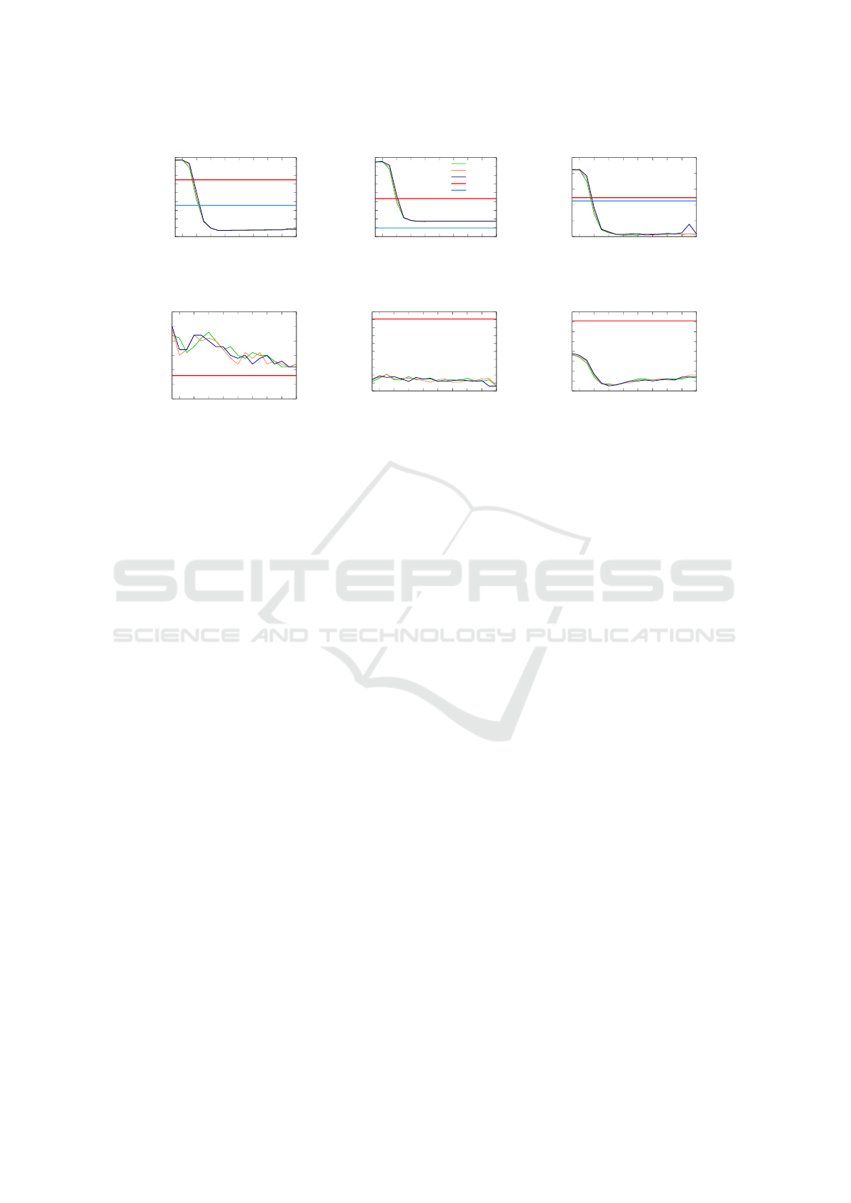
ploying a ﬁxed sized Bloom ﬁlter can help to improve

query performance with low memory overhead. How-

ever, as the performance of the Bloom ﬁlter varies

with its size M, we conducted various experiments

with both partition and routing based Bloom ﬁlter im-

plementations. For the experiments in Figure 5, we

examined both queries on all mentioned data sets. We

have tested the impact of a different number of hash

functions against the baseline, where no Bloom ﬁlter

was used and thus always all workers need to be ac-

tivated. We will only present selected experiments,

due to the large amount of possible experiments. Pre-

sented runtimes are the average of 10 runs, without

the fastest and the slowest runtime. The ﬁrst row of

Figures 5 and 6 shows selected experiments for the

raw storage with only outgoing edges, and the second

row applies our Bloom ﬁlter on top of the fully redun-

dant storage, to show that combining both strategies

can improve our performance even further. Because

of the varying runtime between the testing queries and

on different graphs, we scaled the Y-axis accordingly

for every experiment in Figures 5 and 6.

All ﬁgures from Figure 5, except Figure 5(e),

clearly show the desired results. That is, the big-

ger the Bloom ﬁlter, the bigger is the performance

beneﬁt. Increasing the Bloom ﬁlter size is indirectly

proportional to the expected false positive rate, thus

leading to less unnecessary work. In detail, Fig-

ure 5(b) behaves like anticipated. Adding a Bloom

ﬁlter will increase the performance to allow query

runtimes somewhere between the raw storage and the

fully redundant storage. On top of that, Figures 5(a)

and 5(c) show an improved performance even beyond

the fully redundant storage. The same holds true for

Figures 5(d) and 5(f). Applying our Bloom ﬁlter tech-

nique on top of the fully redundant storage leads to an

additional performance boost, since the Bloom ﬁlter

acts as a secondary index structure. By blooming all

target vertices for every source vertex in a partition,

the Bloom ﬁlter can most certainly reject requests for

edges with a target vertex, which is not present in the

respective partition.

Figure 5(e) is a special case. For smaller Bloom

ﬁlters, the systems performance is slower than us-

Trading Memory versus Workload Overhead in Graph Pattern Matching on Multiprocessor Systems

405

500

1000

1500

2000

2500

3000

3500

4000

4500

Query runtime [ms]

Bloom Filter size [bit]

RRV partitioning

(a) Bib, Q1, BC

200

400

600

800

1000

1200

1400

1600

1800

Query runtime [ms]

Bloom Filter size [bit]

HV partitioning

7 Hashes

8 Hashes

9 Hashes

Unoptimized

Full Redundancy

(b) Bib, Q2, BC

100

150

200

250

300

Query runtime [ms]

Bloom Filter size [bit]

RRV partitioning

690

695

700

705

710

715

720

Query runtime [ms]

RRV partitioning

(d) Uni, Q2, UC

600

610

620

630

640

650

660

670

680

690

700

Query runtime [ms]

Bloom Filter size [bit]

KWay partitioning

(e) Bib, Q2, UC

110

120

130

140

150

160

170

180

190

Query runtime [ms]

Bloom Filter size [bit]

Hash partitioning

(f) Social, Q1, UC

Figure 6: Query Performance with varying Bloom ﬁlter parameters, Bloom ﬁlter implemented with the partitioning infor-

mation. The baseline denotes the performance without a Bloom ﬁlter. BC = Broadcasts with ’OES’ as Unoptimized, UC =

Unicasts with ’Fully redundant’ as Unoptimized

ing the raw storage. Although the query runtime is

consistently decreasing, it barely reaches the baseline

performance, where no Bloom ﬁlter is used. This be-

havior can be explained with the amount of broadcasts

in the system, when only a small number of partitions

contains actual data. Since the Bloom ﬁlter is only

active, after the messages have been sent, we still see

the same amount of messages in the system and the

overhead of checking the Bloom ﬁlter is added on top

of it.

For better comparability, Figure 6 shows the same

experiments as Figure 5, but with the adjusted Bloom

ﬁlter location. Most surprising is the observation, that

avoiding messages is not generally better. For exam-

ple, the experiments of Figures 5(d) and 6(d) show a

better performance, when messages are ﬁltered out in

parallel, instead of avoiding them; the same holds for

Figures 5(e) and 6(e) respectively. This effect can be

explained with the large serial code segment, which

is executed, whenever the Bloom ﬁlter is probed. On

the other hand, the experiments in Figures 6(a) to 6(c)

greatly beneﬁt from the reduced message load. As for

Figure 6(f), we can clearly see that there is an optimal

Bloom ﬁlter size, after which the performance drops,

possibly reasoned by the bigger bitﬁelds, which get

less cache friendly.

5 RELATED WORK

Graph processing is a wide ﬁeld with continuously

ongoing research. Because of the plethora of use

cases, many systems are built to solve a speciﬁc prob-

lem. A comparable system might be Pregel+ (Yan

et al., 2015), which was considered as the fastest

graph engine (Lu et al., 2014). In that system, ev-

ery worker is an MPI process and exchanges mes-

sages. Pregel+ leverages vertex mirroring to distribute

workload for improved performance, which is orthog-

onal to our approach of reducing workload. In our

evaluation, we showed that redundancy introduces a

huge memory overhead for the achieved performance,

compared to our Bloom ﬁlter approach. A more re-

cent system is Turbograph++ (Ko and Han, 2018),

which distributes vertices and edges among multi-

ple machines, where each machine stores the data

on disk. The main difference between our system

and TurboGraph++ is our processing model. Because

of the inherent messaging, our model resembles a

streaming engine, where the data ﬂows from one op-

erator to the next, where invalid intermediate results

get pruned on the ﬂy. The authors of (Neumann and

Weikum, 2009) use a Bloom ﬁlter to avoid construct-

ing full semi-join tables on RDF data graphs, whereas

our approach uses a Bloom ﬁlter to completely elimi-

nate the need to touch a whole data partition.

DATA 2019 - 8th International Conference on Data Science, Technology and Applications

406

6 CONCLUSION

In this paper we have presented measures for trad-

ing storage overhead for workload reduction. Our

key ﬁndings were, that despite being more accu-

rate, fully redundant storage does not yield propor-

tional performance gain, compared to the memory in-

vested. We could show in our evaluation, that our

hand tuned Bloom ﬁlter approach can save a tremen-

dous amount of main memory and still provide rea-

sonable speedups. Considering the huge experimen-

tal space, we envision to continue this research and

combine these ﬁndings with (Krause et al., 2017a),

to built an adaptive system, which can adapt both the

partitioning and the employed Bloom ﬁlter to achieve

optimal performance.

REFERENCES

Bagan, G., Bonifati, A., Ciucanu, R., Fletcher, G. H. L.,

Lemay, A., and Advokaat, N. (2017). gMark:

Schema-driven generation of graphs and queries.

IEEE Transactions on Knowledge and Data Engineer-

ing, 29(4).

Bloom, B. H. (1970). Space/time trade-offs in hash coding

with allowable errors. Communications of the ACM,

13(7).

Borkar, S. et al. (2011). The future of microprocessors.

Commun. ACM, 54(5).

Broder, A. Z. and Mitzenmacher, M. (2003). Survey: Net-

work applications of bloom ﬁlters: A survey. Internet

Mathematics, 1(4).

Decker, S., Melnik, S., van Harmelen, F., Fensel, D., Klein,

M. C. A., Broekstra, J., Erdmann, M., and Horrocks,

I. (2000). The semantic web: The roles of XML and

RDF. IEEE Internet Computing, 4(5).

Granlund, T. (2017). Instruction latencies and

throughput for AMD and Intel x86 processors.

https://gmplib.org/˜tege/x86-timing.pdf.

Hull, T. E. and Dobell, A. R. (1962). Random Number Gen-

erators. SIAM Review, 4.

Karypis, G. and Kumar, V. (1998). A fast and high quality

multilevel scheme for partitioning irregular graphs.

Kissinger, T., Kiefer, T., Schlegel, B., Habich, D., Molka,

D., and Lehner, W. (2014). ERIS: A numa-aware in-

memory storage engine for analytical workload. In In-

ternational Workshop on Accelerating Data Manage-

ment Systems Using Modern Processor and Storage

Architectures - ADMS, Hangzhou, China, September

Ko, S. and Han, W. (2018). Turbograph++: A scalable and

fast graph analytics system. In Proceedings of the In-

ternational Conference on Management of Data, SIG-

MOD Conference, Houston, TX, USA, June 10-15.

Krause, A., Kissinger, T., Habich, D., Voigt, H., and Lehner,

W. (2017a). Partitioning strategy selection for in-

memory graph pattern matching on multiprocessor

systems. In Euro-Par 2017: Parallel Processing -

23rd International Conference on Parallel and Dis-

tributed Computing, Santiago de Compostela, Spain,

August 28 - September 1, Proceedings.

Krause, A., Ungeth

um, A., Kissinger, T., Habich, D., and

Lehner, W. (2017b). Asynchronous graph pattern

matching on multiprocessor systems. In New Trends

in Databases and Information Systems - ADBIS 2017

Short Papers and Workshops, AMSD, BigNovelTI,

DAS, SW4CH, DC, Nicosia, Cyprus, September 24-

27, Proceedings.

Lu, Y., Cheng, J., Yan, D., and Wu, H. (2014). Large-scale

distributed graph computing systems: An experimen-

tal evaluation. PVLDB, 8(3).

Neumann, T. and Weikum, G. (2009). Scalable join pro-

cessing on very large RDF graphs. In Proceedings of

the ACM SIGMOD International Conference on Man-

agement of Data, Providence, Rhode Island, USA,

June 29 - July 2.

Otte, E. and Rousseau, R. (2002). Social network analysis:

a powerful strategy, also for the information sciences.

J. Information Science, 28(6).

Pandis, I., Johnson, R., Hardavellas, N., and Ailamaki, A.

(2010). Data-oriented transaction execution. PVLDB,

3(1).

Pandit, S., Chau, D. H., Wang, S., and Faloutsos, C. (2007).

Netprobe: a fast and scalable system for fraud detec-

tion in online auction networks. In Proceedings of the

16th International Conference on World Wide Web,

Banff, Alberta, Canada, May 8-12.

Paradies, M. and Voigt, H. (2017). Big graph data ana-

lytics on single machines - an overview. Datenbank-

Spektrum, 17(2).

Sutter, H. (2005). The free lunch is over: A fundamental

turn toward concurrency in software. Dr. Dobb’s jour-

nal, 30(3).

Tran, T., Wang, H., Rudolph, S., and Cimiano, P. (2009).

Top-k exploration of query candidates for efﬁcient

keyword search on graph-shaped (RDF) data. In Pro-

ceedings of the 25th International Conference on Data

Engineering, ICDE, March 29 - April 2, Shanghai,

China.

Wood, P. T. (2012). Query languages for graph databases.

SIGMOD Record, 41(1).

Yan, D., Cheng, J., Lu, Y., and Ng, W. (2015). Effec-

tive techniques for message reduction and load bal-

ancing in distributed graph computation. In Proceed-

ings of the 24th International Conference on World

Wide Web, Florence, Italy, May 18-22.

Trading Memory versus Workload Overhead in Graph Pattern Matching on Multiprocessor Systems

407