Sustainable Development Goal Attainment Prediction: A Hierarchical

Framework using Time Series Modelling

Yassir Alharbi

1,3

, Daniel Arribas-Be

and Frans Coenen

Department of Computer Science, University of Liverpool, Liverpool, U.K.

Geographic Data Science Lab., Department of Geography & Planning, University of Liverpool, U.K.

Almahd College Taibah University, Al-Madinah Al-Munawarah, Saudi Arabia

Keywords:

Bottom-up Hierarchical Classiﬁcation, Time Series Forecasting, UN Sustainable Development Goals.

Abstract:

A framework is presented which can be used to forecast weather an individual geographic area will meet its

UN Sustainable Development Goals, or not, at some time t. The framework comprises a bottom up hierar-

chical classiﬁcation system where the leaf nodes hold forecast models and the intermediate nodes and root

node “logical and” operators. Features of the framework include the automated generation of the: associated

taxonomy, the threshold values with which leaf node prediction values will be compared and the individual

forecast models. The evaluation demonstrates that the proposed framework can be successfully employed to

predict whether individual geographic areas will meet their SDGs.

1 INTRODUCTION

In the year 2000, leaders of the world gathered in

the United Nations to ﬁnally agree, after a decade

of conferences and summits, to adopt a set of eight

Millennium Development Goals (MDGs) (United Na-

tions Development programme, 2007). The eight

goals were directed at different aspects of humani-

tarian well being. The success of the MDGs initia-

tive prompted the United Nations (UN) to propose

a further set of seventeen Sustainable Development

Goals (SDGs) in 2015, with an attainment date of

2030. A series of targets and indicators were iden-

tiﬁed and listed in the United Nations’ “Transforming

our World: the 2030 Agenda for Sustainable Devel-

opment” (UN, 2015). An individual goal, a Sustain-

able Development Goals (SDG), is met if the associ-

ated indicator values meet some condition. This paper

presents a framework for predicting whether a given

country (geographic region) will meet its SDGs by a

given date t with reference to the UN SDG dataset,

a publicly available data set which at time of writing

(2019) comprised 1, 083, 975 records.

Whether a country meets its SDGs or not is depen-

dant on whether individual SDGs are met, which in

turn depends on whether the component targets mak-

ing up an individual SDG are met, which also de-

pends on whether particular indicators, sub-indicators

and, in some cases, sub-sub-indicators are met; which

inherently suggests a hierarchical forecasting (classi-

ﬁcation) system. However, unlike established hier-

archical classiﬁcation systems, which work in a top

down manner (Silla and Freitas, 2011), the envisaged

prediction mechanism would work in a bottom-up

manner. In both cases, the objective is to establish the

“class” of an entity with respect to some predeﬁned

hierarchical taxonomy, and in both cases, the classiﬁ-

cation will operate in a level-by-level manner. How-

ever, the branches in the taxonomy in the top down

case represent disjunctions, while the branches in the

bottom up case represent conjunctions. In the top

down case, the identiﬁed path in the hierarchy from

the root node to the leaf node holds the labels to be

assigned to the entity to be classiﬁed; In the bottom-

up case, labels associated with the leaf nodes need

to be established before labels associated with parent

nodes can be established, all the way up to the root

node; The taxonomy in the case of bottom up hierar-

chical classiﬁcation can thus be thought of as a “de-

pendency tree” (Zhang et al., 2018). An alternative

way of differentiating the two approaches is to de-

scribe top down hierarchical classiﬁcation as adopt-

ing a “coarse-to-ﬁne” classiﬁcation approach, whilst

bottom up hierarchical classiﬁcation adopts a “ﬁne-

to-coarse” classiﬁcation approach. It should also be

noted that top-down hierarchical classiﬁcation was

originally proposed as a mechanism for addressing

classiﬁcation problems that featured a large number

Alharbi, Y., Arribas-Be, D. and Coenen, F.

Sustainable Development Goal Attainment Prediction: A Hierarchical Framework using Time Series Modelling.

DOI: 10.5220/0008067202970304

In Proceedings of the 11th International Joint Conference on Knowledge Discovery, Knowledge Engineering and Knowledge Management (IC3K 2019), pages 297-304

ISBN: 978-989-758-382-7

297

of classes. Techniques for top down hierarchical clas-

siﬁcation are well established, techniques for bottom

up hierarchical classiﬁcation have been less well stud-

ied.

In the proposed bottom up framework, each node

will hold a time series forecasting model. At the

root and intermediate nodes, the models will simply

take binary input from their child nodes and apply

a Boolean function to this input, passing the result

to their parent node (or as output in the case of the

root node). At the leaf nodes, the classiﬁcation mod-

els will be more sophisticated addressing individual

indicators, sub-indicators or sub-sub-indicators. The

question to be addressed is then the nature of the fore-

casting models to be held at the leaf nodes. At their

simplest such models would consider a single indica-

tor (sub-indicator or sub-sub-indicator), operating on

the assumption that there is no link between the indi-

cator and other indicators.

The rest of this paper is organised as follows. Sec-

tion 2 presents a brief literature review of the previ-

ous work underpinning the work presented in this pa-

per. The SDG data set is described in further detail in

Section 3. The proposed SDG bottom-up hierarchical

classiﬁcation framework is then presented in Section

4. The evaluation of the proposed framework is dis-

cussed in Section 5. The paper is concluded in Section

6 with a summary of the main ﬁndings.

2 LITERATURE REVIEW

In this section a brief literature review of the work un-

derpinning the SDG prediction framework proposed

in this paper is presented. The literature review com-

mences, sub-section 2.1, with a review of existing

work directed at the SDG challenge. The problem is

essentially a time series forecasting problem; hence a

review of time series forecasting is presented in sub-

section 2.2. As noted in the introduction to this report,

the SDG problem can be couched as a Hierarchical

classiﬁcation problem. Hierarchical classiﬁcation is

therefore discussed in some further detail sub-section

2.3.

2.1 Sustainable Development Goal

Challenge

Many studies have been published on the SDG prob-

lem problem, and the SDG challenge in general. To

monitor the progress of SDGs, the UN publishes a

yearly report (UN, ) to measure the progress towards

the global attainment of the SDGs; the report pro-

vides a good annual general overview. The UN also

publishes statistics used to monitor progress towards

SDG attainment

; this is the input data used with re-

spect to the proposed framework and is therefore dis-

cussed in further detail in Section 3. The majority

of the available literature has been directed at indi-

vidual SDGs. For example, Cuaresma et al. (Cre-

spo Cuaresma et al., 2018) considered the SDG “End

poverty in all its forms everywhere” (SDG 1). The

proposed forecasting mechanism was based on a sin-

gle criteria GDP (Gross Domestic Proﬁt) by using

regression-based estimates. In Shumilo et al. (Shu-

milo et al., 2018) the SDG “Life on land” (SDG 15)

was considered. Here the proposed forecasting mech-

anism was founded on the utilisation of satellite im-

agery by implementing neural networks to classify

forest area. SDG 11 was considered in (Anderson

et al., 2017) using data obtained from air quality sen-

sors installed on data collection satellites.

2.2 Time Series Forecasting

Time series analysis has been the subject of much

research (Konar and Bhattacharya, 2017; Hyndman,

2018). Much of this work has been directed at su-

pervised learning, the mapping of time series to class

labels of some kind (Bagnall et al., 2016). Many

methods have been proposed to predict (forecast) fu-

ture occurrences in time series data, examples in-

clude: Vector Autoregression (Stock and Watson,

2001), Holt Winters Exponential Smoothing (Gelper

et al., 2010) and autoregressive (Gooijer and Hynd-

man, 2006). In the context of SDG prediction a par-

ticular challenge is the nature of the time series data

available; at time of writing (2019) this was limited to

18 observation points per time series.

Any forecasting method, considered in the con-

text of the proposed framework, must therefore be

able to operate using such short time series. From

the literature there are three models that seem appro-

priate: (i) Auto-Regressive Moving Average (Arma)

(Lawrance and Lewis, 1980), (ii) Auto-Regressive

Integrated Moving Average (ARIMA) (Hyndman,

2018), and (iii) Facebook Prophet (Fbprophet) (Tay-

lor and Letham, 2017).

The ARMA model combines autoregression

(Mills, 1990) with a moving average model. It can

be expressed as shown in Equation 1, where φ is the

auto regressive models parameter, θ is the moving av-

erage, c is a constant and ε is the error terms.

= c + ε

∑

i=1

t−i

∑

i=1

t−i

(1)

https://unstats.un.org/SDGs/indicators/database/

KDIR 2019 - 11th International Conference on Knowledge Discovery and Information Retrieval

298

The ARIMA time series forecasting model is

a generalisation of the ARMA model (Hyndman,

2018). It can be expressed as shown in Equation 2,

where t is a temporal index, u is the mean term, B is

the backshift operator, φ(B) is the autoregressive op-

erator, θ(B) is the moving average operator, and a

the independent disturbance or the random error.

(1 − B)

= µ +

θ(B)

φ(B)

(2)

Fbprophet is an additive regression model, di-

rected at non-linear time series forecasting, developed

by Facebook (Taylor and Letham, 2017). Fbprophet

operates by decomposing a given time series into

three different components, the “trend”, “seasonal-

ity”, and “holidays” components, and includes an er-

ror term as shown in Equation 3 where g(t) is the

trend, s(t) is the the periodic change, h(t) is the sea-

sonality effect and ε is the parametric assumption.

The result is a model that is robust to short time se-

ries and randomness in the observation points.

y(t) = g(t)+ s(t) + h(t) + ε

(3)

An alternative to the above is to consider forecast-

ing methods directed at hierarchical time series such

as those proposed in (Wickramasuriya et al., 2018)

and (Hyndman, 2018), applicable where the time se-

ries under consideration naturally divided hierarchi-

cally. The example given in (Athanasopoulos et al.,

2009) is forecasting tourism in Australia. However,

given that the available SDG time series are already

very short the potential for a hierarchical division of

these time series is very limited and unlikely to prove

successful.

A further disadvantage of short time series fore-

cast model generation is that there is very little op-

portunity for taking the presence of noise into con-

sideration. It is argued that inaccuracy in time series

forecasting is directly related to the amount of noise

in the data; the proportion of noise in short time series

is often higher than in long time series (Hyndman and

Kostenko, 2007). In the context of the SDG applica-

tion, it is unclear how much noise there is, or how this

might be deﬁned; it can be argued that, there is no

spurious data and hence no noise. Whatever the case,

given a collection of short time series the interaction

between the different time series may be utilised, al-

though this is not considered in this paper.

2.3 Hierarchical Classiﬁcation

As noted in the introduction to this paper, hierarchical

classiﬁcation is a type of supervised learning where

the output of the classiﬁcation is derived from a hi-

erarchical class taxonomy (Silla and Freitas, 2011).

There are many methods directed at top-down classi-

ﬁcation, examples can be found in (Dangerﬁeld and

Morris, 1992) and (Edwards and Orcutt, 1969). As

far as the authors are aware there has been little

work directed at bottom-up hierarchical classiﬁcation

founded on a taxonomy. In (Rostami-Tabar et al.,

2013) a new approach, called grouped time series,

was discussed. This approach was applicable given

an application where the required time series forecast-

ing is to be conducted used multiple levels of granu-

larity. For example in a warehouse stock forecasting

application where there are thousands of products ar-

ranged according to a hierarchical categorisation; not

quite the same as the SDG challenge but of interest

because of its hierarchical nature.

3 THE SUSTAINABLE

DEVELOPMENT GOALS DATA

SET

Each of the UN’s 17 SDGs has between 3 and 13 tar-

gets, and each target, in turn, has a number of indi-

cators associated with it. In most cases, the indica-

tors have sub-indicators, and even sub-sub-indicator

(Sapkota, 2019). An illustration of the SDG hier-

archical structure is given in Figure 1. With refer-

ence to the ﬁgure, the time series forecast models will

be held at the leaf nodes, while the remaining inter-

mediate nodes and the root node will hold “logical

and” functions. For ease of understanding a num-

bering system has been adopted to identify individual

indicators, hg,t, i, s1, s2i (goal, target, indicator, sub-

indicator, sub-sub-indicator), for example the identi-

ﬁer [1.1.1.1.1] indicates: Goal1, Target 1, Indicator 1,

sub-indicator1, sub-sub-indicator 1.

The SDG data set is publicly available from the

SDG website

. At time of writing (2019) the data set

spanned an 18 year period. The SDG data set is rel-

atively large, 500MB, and is comprised of 1, 083, 975

records holding statistical SDG information covering

individual geographic areas. An example record is

given in Table 1. Here the indicator is 3.7.2, “Adoles-

cent birth rate (aged 10-14 years; aged 15-19 years)

per 1,000 women in that age group”, and the sub-

indicator (series description) is Adolescent birth rate

(per 1,000 women aged 15-19 years). The major-

ity of geographic areas considered are countries that

currently exist, 195 of them. The remainder com-

prise countries that currently are no longer in exis-

https://unstats.un.org/SDGs/indicators/database/

Sustainable Development Goal Attainment Prediction: A Hierarchical Framework using Time Series Modelling

299

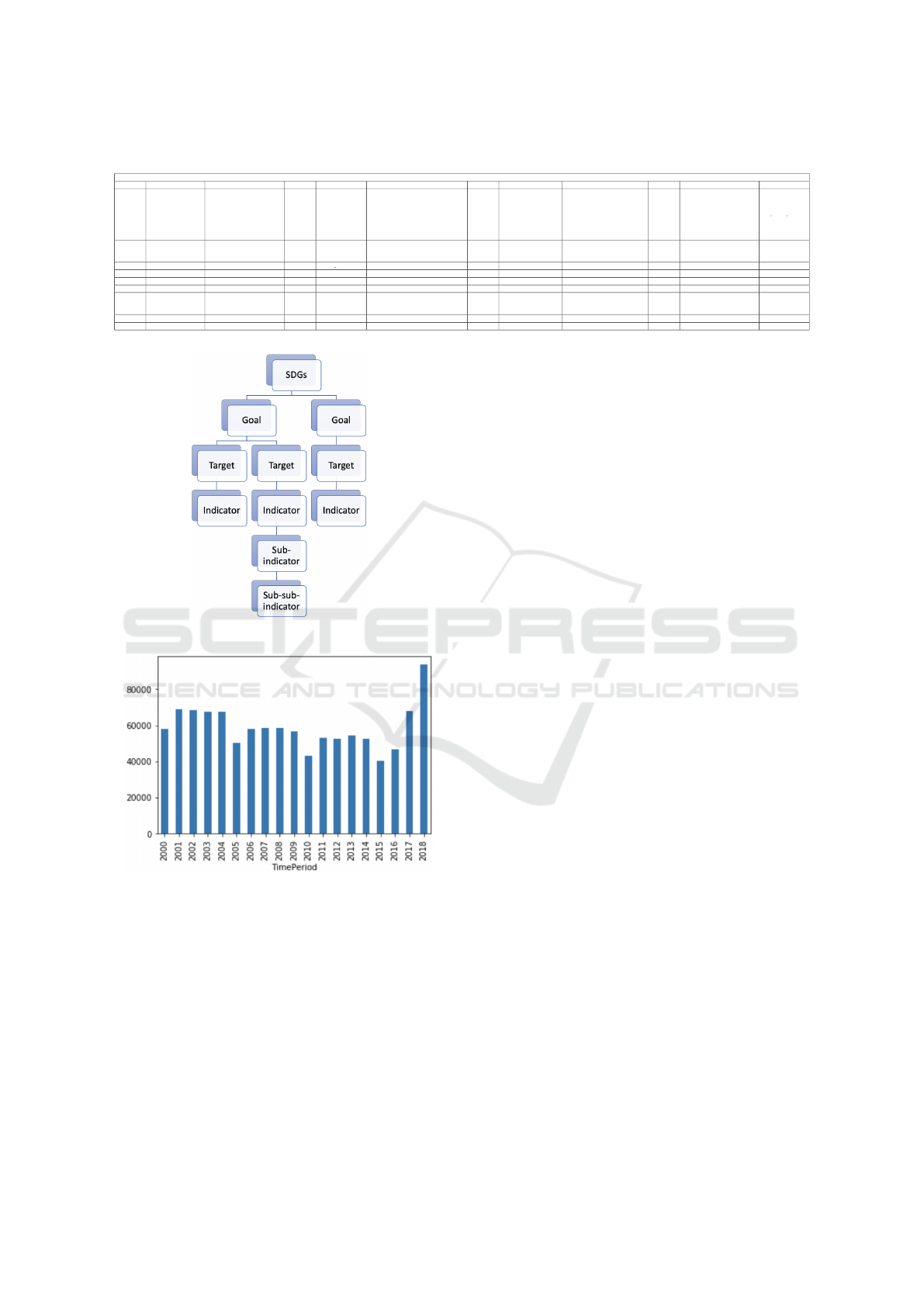
Table 1: SDG example record.

Record sample

Att Num Label Value Att Num Label Value Att Num Label Value Att Num Label Value

1 Goal

Goal 3. Ensure healthy lives

and promote well-being for

all at all ages

2 Target

By 2030, ensure universal

access to sexual and reproductive

health-care services, including

for family planning, information

and education, and the integration of

reproductive health into

national strategies and programmes

3 Indicator

3.7.2 Adolescent birth rate

(aged 10–14 years; aged

15–19 years) per 1,000 women

in that age group

4 SeriesCode SP DYN ADKL

5 SeriesDescription

Adolescent birth rate

(per 1,000 women aged

15-19 years)

6 GeoAreaCode 818 7 GeoAreaName Egypt 8 TimePeriod 2001

9 Value 47 10 Time detail nan 11 Source nan 12 FootNote nan

13 Nature nan 14 Units nan 15 Age 15-19 16 Bounds nan

17 Cities nan 18 Education level nan 19 Freq nan 20 Hazard type nan

21 IHR Capacity nan 22 Level/Status nan 23 Location nan 24 Migratory status nan

Mode of

transportation

nan 26

Name of

international

institution

nan 27

name of non-

communicable

disease

nan 28 Quantile nan

29 Reporting Type nan 30 Sex Female 31 Tarif regime (status) nan 32

Type of Mobile technology

nan

33 Type of occupation nan 34 Type of product nan 35 Type of skill nan 36 Type of Speed nan

Figure 1: SDG Hierarchy.

Figure 2: Histogram summarising number of SDG absent

and missing data values per sample year.

tence and geographic groupings of countries. Each

record references a particular time stamp (year), ge-

ographical area and indicator (sub -indicator or sub-

sub-indicator). The data is organised according to

36 columns (attributes) these are listed in Table 1.

The ﬁrst three columns list the goal, target and in-

dicator referenced by each record. The geographi-

cal area ID and name are given in Columns 6 and 7

and the associated time stamp in column 8. The re-

maining 29 columns give additional information con-

cerning whether a record referrers to a sub-indicator

or a sub-sub-indicator or not, and relevant values. In

many cases the attribute referenced by the column is

not applicable, hence the value is absent. For example

the last attribute, Column 36, refers to internet speed

which is irrelevant with respect to most indicators. In

other cases the the column is applicable, but the value

is missing. Hence the data set features both “absent”

and “missing” values”; a summary of the number of

absent and missing values featured in the data set is

given in Figure 2.

As noted above the data set spans an 18 year pe-

riod, thus for a given geographic area and a given in-

dicator (sub-indicator or sub-sub-indicator) there will

be a time series comprised of a maximum of 18 points

(values). There are records where the time series only

feature a small number of points, the remaining val-

ues being missing.

The SDG data set D, as described above, is there-

fore comprises of a single table measuring r × |A|,

where r is the number of records and |A| is the size

of the attribute set (the number of columns). At time

of writing r = 1, 083, 975 and |A| = 36. To gener-

ate the desired forecast models the data set D had to

be “reshaped” (Wang et al., 2019) to give a data set

= e × y where e is the number of leaf nodes that

will feature in the SDG hierarchy, and y is the number

of years for which data is available. At time of writ-

ing D = 1803096 (18 × 128429 and y = 18; it is antic-

ipated that y will increase year-by-year as further data

becomes available. The data set D

holds numeric val-

ues only. In effect each row in D

is a time series

, v

, . . . , v

} which in turn can be used to build the

desire forecast models. As noted above the data set

spans an 18 year period, thus for a given geographic

area and a given indicator (sub-indicator or sub-sub-

indicator) there will be a time series comprised of a

maximum of 18 points (values). There are records

where the time series only feature a small number of

points, the remaining values being missing.

KDIR 2019 - 11th International Conference on Knowledge Discovery and Information Retrieval

300

4 THE SDG PREDICTION

FRAMEWORK

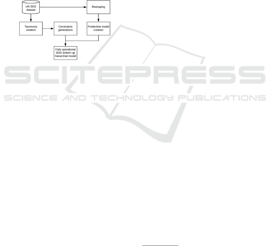
This section details the SDG Prediction Framework.

There are three aspects to the Prediction Framework:

(i) the generation of the taxonomy, (ii) the generation

of the associated constraints to be embedded in the

framework and (iii) prediction model generation. The

ﬁrst two are generic processes independent of the geo-

graphic region of interest; the third is a geographic re-

gion dependent process that will be repeated for each

geographic region to be considered. Each is discussed

in further detail in the following three sub-sections.

A schematic of the proposed SDG framework is pre-

sented in Figure 3.

Figure 3: System overview.

4.1 SDG Taxonomy Generation

Hierarchical classiﬁcation (top-down or bottom-up)

requires a taxonomy and associated hierarchy. In

many cases of top-down hierarchical classiﬁcation,

the hierarchy and taxonomy are easily deﬁned and

are often quite trivial. In the case of the SDG hier-

archy, the hierarchy and taxonomy are substantial as

indicated in Figure 1. Further, the UN does not pro-

vide a taxonomy for the data. Therefore the taxon-

omy and hierarchy need to be extracted from D (the

UN SDG data set). Hand-crafting of the taxonomy

and hierarchy was clearly not a desirable option, as it

would be time-consuming and prone to error; there is

also the potential that the UN may change elements

of the SDGs, or add a completely new goal or edit

an existed one. An automated approach to generat-

ing the taxonomy and hierarchy was therefore seen as

desirable. A Hierarchical Taxonomy Generator was

developed for this purpose, the input for which was

the raw SDG data for all geographical regions. This

was developed using the Python Pandas library for

data manipulation and analysis, speciﬁcally the cross-

tabulation (Crosstab) function included in the Pandas

library. Now Crosstab is used to do contingency ta-

ble. So before using the method to produce the taxon-

omy, some columns must be removed from the data

set such as Value and dates. We only keep what is im-

portant to produce the hierarchical representation of

the data set; we also need a unique id for each differ-

ent combination. So we do summation operation in

all the columns together to create a unique ID. now

we use the crosstab with the following argument

This allowed for the automated generation of SDGs

taxonomy from D from which the associated hierar-

chy could be inferred. A fragment of the generated

taxonomy is shown in Table 2,

4.2 Threshold Generation

Each node in the SDG hierarchy (Figure 1) has a

boolean condition associated with it. At the root and

intermediate nodes the conditions are expressed sim-

ply as “logical and” functions; if all the inputs have

the value True the output value will be True, and

False otherwise. At the leaf nodes, the conditions are

more complex and are outlined in the SDG Handbook

(Sapkota, 2019). These are typically expressed in the

form of some conditional operator, such as greater

than (>), less than (<) or equal to (=), some thresh-

old σ. The challenge is that the σ values to be associ-

ated with the leaf nodes are not included in D and

are not speciﬁed in (Sapkota, 2019). Instead, they

are published separately in (UN, 2017). However,

in (UN, 2017) some of the thresholds are not math-

ematically deﬁned. A solution, in the context of the

proposed hierarchical framework, was available in the

(Lozano et al., 2018) where the authors published a

mathematical interpretation for the health-related tar-

gets from the SDG published target goals document.

The same methodology was replicated and used upon

all other targets manually. The generated thresholds

were added to the SDG Taxonomy produced by the

Hierarchical Taxonomy Generator described above in

sub-section 4.1, a fragment of the updated SDG tax-

onomy, with threshold conditions and expected com-

pliance date, is given in Table 2. Once the full SDG

Taxonomy had been generated, it could be used to

generate the required SDG hierarchy automatically.

4.3 Forecast Model Generation

As noted above, each leaf nodes in the hierarchy will

hold a forecast model. The forecast models at the

leaf nodes are required to predict what the value as-

sociated with the indicator in question will be and

then to determine whether that value meets its spec-

iﬁed threshold value σ or not. However, unlike the

pd.crosstab([dataset.Goal, dataset.Target,

dataset.Indicator, dataset.SeriesDescription,

dataset.SeriesCode], [dataset.TimePeriod])

Sustainable Development Goal Attainment Prediction: A Hierarchical Framework using Time Series Modelling

301

Table 2: Fragment of SDGs taxonomy and thresholds.

Goal Target Indicator Series Description Series Code Threshold Date

1 1.1 1.1.1

Proportion of population below international poverty line (%) SI POV DAY1 ≤ 0.05% 2030

Employed population below international poverty line by sex and age(%)

SI POV EMP1 15-24 MALE ≤ 0.05% 2030

SI POV EMP1 MALE 15+ ≤ 0.05% 2030

SI POV EMP1 MALE 25+ ≤ 0.05% 2030

SI POV EMP1 BOTHSEX 15+ ≤ 0.05% 2030

SI POV EMP1 BOTHSEX 25+ ≤ 0.05% 2030

SI POV EMP1 BOTHSEX 15-24 ≤ 0.05% 2030

SI POV EMP1 FEMALE 15+ ≤ 0.05% 2030

SI POV EMP1 FEMALE 25+ ≤ 0.05% 2030

SI POV EMP1 FEMALE 15-24 ≤ 0.05% 2030

SDG hierarchy, generated as described above, the na-

ture of the forecast models are speciﬁc to individual

geographic regions and thus each needs to be gen-

erated on a “as required” basis. The forecast mod-

els held at the leaf nodes were generated using the

available data for each indicator (sub-indicator or sub-

sub-indicator) associated with each geographic area

included in the SDG data set, e = 128429 of them.

A number of forecast model generation mechanisms

were considered, as noted in sub-section 2.2: (i) Auto

Regression Moving Average (ARMA) (Lawrance and

Lewis, 1980), (ii) Auto-Regressive Integrated Moving

Average (ARIMA) (Kinney, 1978) and (iii) Facebook

Prophet (Fbprohphet) (Taylor and Letham, 2017).

5 EVALUATION

The evaluation of the proposed framework is pre-

sented in this section. The evaluation comprised two

elements: (i) evaluation of the forecast models and (ii)

evaluation of the the framework as a whole.

5.1 Forecasting Evaluation

As noted above, three forecast model generators were

considered: (i) ARMA, (ii) ARIMA and (iii) Fbproh-

phet. The evaluation metrics used were: Root Means

Square Error (RMSE) and Means Absolute Percent-

age Error (MAPE) (Hyndman and Koehler, 2006).

RMSE is calculated as shown in Equation 4 where

f is the forecasted value and o is the observed value.

RMSE provides results with the same unit as the fore-

casted values, it is therefore easy to compare RMSE

values generated by alternative forecasting methods,

however it is not an intuitive measure. MAPE is cal-

culated as shown Equation 5 where f is the fore-

casted value and o is the observed value. MAPE of-

fers an easy to understand forecasting error expressed

in terms of a percentage.

RMSE =

( f − o)

(4)

MAPE(

∑

o-f)

) ∗ 100 (5)

For the evaluation SDG Target 3.2, “By 2030, end

preventable deaths of newborns and children under

5 years of age, with all countries aiming to reduce

neonatal mortality to at least as low as 12 per 1,000

live births and under-5 mortality to at least as low as

25 per 1,000 live births”, was selected, together with

the geographic area Egypt. This was selected because

a complete set of data points was available for this

target-geographic location pairing. Target 3.2 com-

prised six indicators; the associated time series are

given in Figure 4. The forecast models were trained

using the ﬁrst seventeen data points and used to pre-

dict the eighteenth (2018) value. The accuracy of the

prediction was measured using RMSE and MAPE.

The results are given in Table 3. From the table, it can

be seen that the Fbprophet prediction model produced

the best results. For example in the case of forecasting

“Neonatal mortality rate (deaths per 1,000 live birth)”

the RMSE score was 0.55 using ARIMA, 5.24 using

ARMA and 0.016 using Fbprophet. Figure 5 shows

the output using Fbprophet.

Figure 4: Indicator time series for Target 3.2.

5.2 Framework Evaluation

To evaluate the utility of the proposed SDG frame-

work the geographic area Egypt was again used to-

gether with SDG Target 3.2. The framework was then

KDIR 2019 - 11th International Conference on Knowledge Discovery and Information Retrieval

302

Table 3: Evaluation results using three different forecast model generators.

Indicator

ARIMA

MAPE

ARIMA

RMSE

ARMA

MAPE

ARMA

RMSE

Fbprophet

MAPE

Fbprophet

RMSE

Infant deaths (number) (Male) 4.475% 5115 13.376% 14258 2.188% 2688

Infant mortality rate (deaths per 1,000 live births) (Male) 1.121% 0.771 0.392% 24 0.012% 0.016

Under-ﬁve deaths (number) 6.197% 8432 16.130% 19975 1.852% 2755

Under-ﬁve mortality rate, by sex (deaths per 1,000 live births) 1.219% 1.015 43.846% 31.661 0.006% 0.010

Neonatal mortality rate (deaths per 1,000 live births) 4.410% 0.591 41.260% 5.249 0.079% 0.016

Neonatal deaths (number) 6.339% 2190 16.472% 5423 0.153% 66.095

Table 4: Framework evaluation using Target 3.2 and the geographic area Egypt.

Goal Series Description Series Code Initial Value Prediction Threshold value Result

3.2

Neonatal mortality rate (deaths per 1,000 live births) SH DYN NMRT BOTHSEX <1M 12.5 13.17215962 <=12 Not Met

Under-ﬁve deaths (number)

SH DYN MORTN MALE <5Y 32537 35278.79895 <=25% Not Met

SH DYN MORTN BOTHSEX <5Y 59728 63777.62493 <=25% Not Met

SH DYN MORTN FEMALE <5Y 27191 30430.79312 <=25% Not Met

Infant deaths (number)

SH DYN IMRTN MALE <1Y 27957 31526.79254 <=25% Not Met

SH DYN IMRTN BOTHSEX <1Y 50924 57755.00977 <=25% Not Met

SH DYN IMRTN FEMALE <1Y 22967 24871.78097 <=25% Not Met

Neonatal deaths (number) SH DYN NMRTN BOTHSEX <1M 31796 32688.55331 <=25% Not Met

Under-ﬁve mortality rate, by sex (deaths per 1,000 live births)

SH DYN MORT MALE <5Y 25.1 25.05650949 <=25% Not Met

SH DYN MORT BOTHSEX <5Y 23.7 25.9189049 <=25% Not Met

SH DYN MORT FEMALE <5Y 22.3 26.04007075 <=25% Not Met

Infant mortality rate (deaths per 1,000 live births)

SH DYN IMRT MALE <1Y 21.4 23.6886514 <=25% Not Met

SH DYN IMRT BOTHSEX <1Y 20.1 21.0875916 <=25% Not Met

SH DYN IMRT FEMALE <1Y 18.7 20.00149873 <=25% Not Met

Figure 5: Forecasted values for Target 3.2.

used to automatically predict whether the target will

be met by 2030, as speciﬁed in the UN Agenda for

Sustainable Development. Target 3.2, as noted above,

encompasses six indicators, six forecast models were

therefore generated using Fbprophet (because earlier

evaluation, reported on in sub-section 5.1, had shown

this produced best results). The prediction models

were trained using the ﬁrst eighteen data points and

then used to predict the 2030 values which were then

used to automatically determine, using the frame-

work, whether the indicators were met, or not, by

comparing the forecasted values with the appropriate

threshold value. In the case of Target 3.2, for the SDG

to be met in 2030, all forecasted values must be less

the 25% of the benchmark value for the year 2015.

The results are presented in Table 4. From the ta-

ble, it can be seen that in the case of the geographic

area Egypt and Target 3.2 the target will not be met

by 2030. However, if the “trend” for each indicator

is examined, as shown in Figure 5, it can be seen that

the SDG will be met at some time in the future.

5.3 Framework Visualisation

An additional feature of the proposed SDG frame-

work is that it includes a visualisation of predictions

in the form of dendrograms generated using the D3.js

JavaScript library (Bostock et al., 2011). The predic-

tion visualisation for Target 3.2, with respect to the

geographic area of Egypt, is given in

6 CONCLUSION

A framework has been presented for predicting

whether individual geographic areas will meet their

UN SDGs at a given time t. The framework com-

prises a bottom up classiﬁcation hierarchy where the

leaf nodes hold predictors founded on time series data

and the intermediate nodes and root node simple “log-

ical and” operators. A feature of the framework is

that the required hierarchical classiﬁcation taxonomy

and threshold values to be held at leaf nodes (with

which predicted values are compared) are both gen-

erated automatically. For individual geographic areas

individual time series-based predictors are required,

these are also generated in an automated manner. The

framework was evaluated by considering a number of

http://tiny.cc/nz8i9y

Sustainable Development Goal Attainment Prediction: A Hierarchical Framework using Time Series Modelling

303

prediction models, and by using it to predict whether

individual geographic areas would meet their targets

by 2030 as speciﬁed in the UN Agenda for Sustain-

able Development. The best prediction model was

found to be Facebook’s Fbprophet. The evaluation

indicated that the proposed framework could be suc-

cessfully employed to predict whether geographic ar-

eas would meet their targets or not.

REFERENCES

Anderson, K., Ryan, B., Sonntag, W., Kavvada, A., and

Friedl, L. (2017). Earth observation in service of

the 2030 agenda for sustainable development. Geo-

spatial Information Science, 20(2):77–96.

Athanasopoulos, G., Ahmed, R. A., and Hyndman, R. J.

(2009). Hierarchical forecasts for australian domestic

tourism. Int. J. Forecast.

Bagnall, A., Lines, J., , Hills, J., and Bostrom, A. (2016).

Time-series classiﬁcation with cote: The collective of

transformation-based ensembles. IEEE 32nd (ICDE).

Bostock, M., Ogievetsky, V., and Heer, J. (2011). D3 data-

driven documents. IEEE Transactions on Visualiza-

tion and Computer Graphics, 17(12):2301–2309.

Crespo Cuaresma, J., Fengler, W., Kharas, H., Bekhtiar, K.,

Brottrager, M., and Hofer, M. (2018). Will the sustain-

able development goals be fulﬁlled? assessing present

and future global poverty. Palgrave Communications.

Dangerﬁeld, B. J. and Morris, J. S. (1992). Top-down or

bottom-up: Aggregate versus disaggregate extrapola-

tions. Int. J. Forecast, 8(2).

Edwards, J. B. and Orcutt, G. H. (1969). Should aggrega-

tion prior to estimation be the rule? The Review of

Economics and Statistics, 51(4):409–420.

Gelper, S., Fried, R., and Croux, C. (2010). Robust fore-

casting with exponential and holt–winters smoothing.

Journal of Forecasting.

Gooijer, J. G. D. and Hyndman, R. J. (2006). 25 years of

time series forecasting. Int. J. Forecast.

Hyndman, R. J. (2018). Forecasting: principles and prac-

tice.

Hyndman, R. J. and Koehler, A. B. (2006). Another look at

measures of forecast accuracy. Int. J. Forecast.

Hyndman, R. J. and Kostenko, A. V. (2007). Minimum sam-

ple size requirements for seasonal forecasting models.

foresight.

Kinney, W. R. (1978). Arima and regression in analytical

review: An empirical test. The Accounting Review.

Konar, A. and Bhattacharya, D. (2017). Time-series pre-

diction and applications : a machine intelligence ap-

proach. Intelligent systems reference.

Lawrance, A. J. and Lewis, P. A. W. (1980). The ex-

ponential autoregressive-moving average earma(p,q)

process. Journal of the Royal Statistical Society: Se-

ries B (Methodological), 42(2):150–161.

Lozano, R., Fullman, N., Abate, D., Abay, S., Abbafati, C.,

Abbasi, N., Abbastabar, H., Abd-Allah, F.,

Arnl

ov, J.,

and Murray, C. J. L. (2018). Measuring progress from

1990 to 2017 and projecting attainment to 2030 of the

health-related sustainable development goals for 195

countries and territories: a systematic analysis for the

global burden of disease study 2017. The Lancet.

Mills, T. C. (1990). Time series techniques for economists.

Cambridge : Cambridge University Press, 1990.

Rostami-Tabar, B., Babai, M. Z., Syntetos, A. A., and Ducq,

Y. (2013). Forecasting aggregate arma(1,1) demands:

Theoretical analysis of top-down versus bottom-up.

Sapkota, S. (2019). E-Handbook on Sustainable Develop-

ment Goals. United Nations.

Shumilo, L., Kolotii, A., Lavreniuk, M., and Yailymov,

B. (2018). Use of land cover maps as indicators for

achieving sustainable development goals.

Silla, C. N. and Freitas, A. A. (2011). A survey of hierarchi-

cal classiﬁcation across different application domains.

Data Mining and Knowledge Discovery, 22:31–72.

Stock, J. H. and Watson, M. W. (2001). Vector autoregres-

sions. Journal of Economic Perspectives, (4).

Taylor, S. J. and Letham, B. (2017). Forecasting at scale.

The American Statistician.

UN. The Sustainable development goals report 2018.

UN (2015). Transforming our world: the 2030 agenda

for sustainable development. Working papers, eSo-

cialSciences.

UN (2017). Tier classiﬁcation for global sdg indicators.

United Nation.

United Nations Development programme (2007). Millen-

nium Development Goals.

Wang, E., Cook, D., and Hyndman, R. J. (2019). A new tidy

data structure to support exploration and modeling of

temporal data. arXiv e-prints, page arXiv:1901.10257.

Wickramasuriya, S. L., Athanasopoulos, G., and Hyndman,

R. J. (2018). Optimal forecast reconciliation for hier-

archical and grouped time series through trace mini-

mization. Journal of the American Statistical Associ-

ation.

Zhang, C., Tao, F., Chen, X., Shen, J., Jiang, M., Sadler,

B., Vanni, M., and Han, J. (2018). Taxogen: Unsuper-

vised topic taxonomy construction by adaptive term

embedding and clustering.

KDIR 2019 - 11th International Conference on Knowledge Discovery and Information Retrieval

304