Neural Models for Benchmarking of Truck Driver Fuel Economy
Performance
Alwyn J. Hoffman
School of Electrical, Electronic and Computer Engineering, North-West University, Potchefstroom, South Africa
Keywords: Fuel Economy, Truck Driver, Performance Benchmarking, Generalized Regression Neural Network,
Multilayer Perceptron.
Abstract: The transport industry is a primary contributor towards emissions that impact climate change. Fuel economy
is also of critical importance to the profitability of road freight transport operators. Empirical evidence
identified a variety of factors impacting fuel consumption, including route inclination, payload and truck
driver behaviour. This creates the need for accurate fuel usage models and objective methods to distinguish
the impact of drivers from other factors, in order to enable reliable driver performance assessment. We
compiled a data set for 331 drivers completing 7332 trips over 21 routes to obtain evidence of the impact of
route, payload and driver behaviour on fuel economy. We then extracted various regression and neural models
for fuel economy and used these models to remove the impact of route inclination and payload, allowing the
impact of driver performance to be measured more accurately. All models demonstrated significant out-of-
sample predictive ability. Neural models in general outperformed regression models, while amongst neural
models radial basis models slightly outperformed multi-layer perceptron models. The significance of
compensating for factors not controlled by the driver was verified by demonstrating large differences in driver
performance ranking before and after compensating for route inclination and payload.
1 INTRODUCTION
The contribution of the transport sector towards
greenhouse gas emissions has been widely researched
and is estimated at around 29% of all emissions caused
by human activities (United States Environmental
Protection Agency, 2019). While the contribution of
passenger vehicles towards GHG emissions is
expected to be gradually eliminated over the next few
decades through a transition to electric vehicles and
clean production of electricity, this transition will be
more challenging for long haul freight trucks, due to
the large distances covered by these vehicles. Heavy-
duty vehicle GHG EPA regulations are projected to
reduce CO
2
emissions by about 270 million metric tons
over the life of vehicles built under the EPA program,
saving about 530 million barrels of oil. The proposed
program includes standards that would further reduce
GHG emissions and improve the fuel efficiency of
medium and heavy-duty trucks (United States
Environmental Protection Agency, 2019).
While these efforts towards reducing the
environmental impact of long haul trucks should be
encouraged, road freight transport still remains an
essential element of the global economy. This is
specifically relevant in regions with limited availability
of rail infrastructure (Hoffman, 2010); for example
road transport is responsible for 76% of cargo
movement in South Africa; this figure is even higher in
other African countries (Havenga, 2013). Compared
to the rest of the world the cost of transport in Africa is
much higher as a fraction of the total cost of delivered
goods - 18% compared to a global average of less than
10% (Anon., 2014). Fuel cost is the single biggest
contributor to the cost of road transport operations,
representing approximately 40% of operating costs
(Naidoo, 2013). Fuel economy is therefore a critical
element to be managed by road freight transport
operators to ensure continued profitability in a very
competitive industry.
Historical research in the field of fuel consumption
modeling identified the primary factors that impact on
consumption; this includes driver proficiency, payload
and route inclinations (Weille, 1966) (Biggs, 1988)
(Bennett and Greenwood, 1995). Much of the work in
this field focused on the modeling of fuel consumption
in terms of engine characteristics and driving style
(Rakha and Wang, 2017) (Delgado, et al., 2011). Other
studies applied a Big Data approach to large vehicle
fleets, mostly driving on flat roads and at constant
speeds (Perrottaa, et al., 2019) as well as the use of
Hoffman, A.
Neural Models for Benchmarking of Truck Driver Fuel Economy Performance.
DOI: 10.5220/0008065703790390
In Proceedings of the 11th International Joint Conference on Computational Intelligence (IJCCI 2019), pages 379-390
ISBN: 978-989-758-384-1
Copyright
c
 2019 by SCITEPRESS – Science and Technology Publications, Lda. All rights reserved
379

telematics solutions to improve fuel consumption
(Hoffman and Van der Westhuizen, 2014).
The use of neural networks to model the fuel
economy of trucks has been the topic of several
research studies (Zhigang Xu, 2018) (Jian-Da Wu,
2012) (Elnaz Siami-Irdemoosa, 2015) (Hassanean S.H.
Jassim, 2018). In all of these studies one of the
objectives was to identify techniques that will provide
the most accurate modeling of fuel economy in terms
of the input factors mentioned above. While
satisfactory results were achieved through the research
efforts listed above, none of those studies tried to
remove the contributions of factors not controlled by
the driver, like route inclinations and payload, before
assessing the performance of the driver. This is of
critical importance, as the only factors that can be
readily influenced to reduce emissions and fuel costs
without negatively impacting the economic function
fulfilled by transport is the behavior of the driver.
Many road transporters offer schemes of incentives
and penalties for fuel efficient driving behavior. This
creates the need for an accurate and objective method
to distinguish the impact of drivers from other factors,
in order to enable fair and consistent driver
performance evaluations.
In previous work we developed linear and nonlinear
regression fuel economy models for long haul freight
trucks using route inclination and payload as
explanatory variables (Hoffman and Van der
Westhuizen, 2019). We also used these models to
evaluate driver fuel economy performance after
compensating for factors not controlled by the driver
(Hoffman and Van der Westhuizen, 2019). In the
absence of such performance corrections, drivers are
assessed by simply calculating their average fuel
economy over all trips, completed over a variety of
routes and carrying varying payloads. This may lead
to inaccurate outcomes as not all drivers are employed
on identical sets of routes driving trucks carrying
identical payloads. The primary purpose of this paper
is to improve on the modelling abilities of regression
models by employing various neural network
architectures. In this study we included radial basis
networks and multilayer perceptron networks.
Based on available evidence we state the hypothesis
that the presence of factors not under the control of the
truck driver, like route inclinations and payload
differences, will significantly impact the performance
outcomes for truck drivers if not properly compensated
for. In order to prove our hypothesis, we will extract
regression and neural models to quantify the impact on
fuel economy of factors not controlled by drivers.
These models will then be used to remove the impact
of such factors in order to arrive at a residual fuel
economy from which the impact of route and payload
has been removed and that is mainly determined by
driver performance. This is expected to produce a
performance measure that is more reliable than a
simple average of the original fuel economy over all
driver trips and that can be used to assess driver
performance more objectively.
We then compare the performance of drivers prior
to model correction with driver performance after
applying such correction. For this purpose, we defined
two measures of driver performance: the first is
whether the driver performed above or below the
average performance measured over all drivers; the
second is the ranking achieved by each driver when
sorting the performance of all drivers from best to
worst. In addition, we also investigate the extent to
which driver identity and driver behaviour can be used
to model the above residual fuel economy. In each case
the abilities of the different modelling techniques will
be compared in terms of their out-of-sample abilities to
correctly predict fuel economy and residual fuel
economy.
The rest of the paper is structured as follows:
section 2 describes the process to collect a
representative set of fuel consumption data, and
describes the different routes that were covered by the
available data set. In section 3 we extract statistical
measures of fuel economy for the population as well as
per route and driver to provide evidence of the need for
a driver performance model. Section 4 focuses on the
extraction of empirical models that will allow us to
isolate the impact of the driver on fuel consumption. In
section 5 we estimate the impact of model
compensation on driver performance measurement. In
section 6 we conclude and make recommendations for
future research work.
2 COLLECTION OF FUEL
CONSUMPTION AND INPUT
FACTOR DATA
The purpose of our fuel usage data collection exercise
was to ensure that we cover all the aspects to be
investigated in this study. We collected data from a
fleet of 468 vehicles that cover most of the major routes
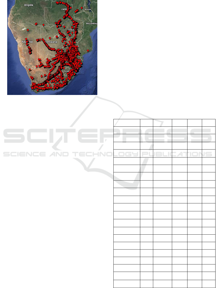
in Southern Africa, as displayed in Figure 1 below.
This allowed us to generate a significant amount of
statistics on routes that include widely ranging
inclinations (e.g. relatively flat from Johannesburg to
Cape Town versus uphill and downhill from Durban to
Johannesburg and back where the Drakensberg
mountain range has to be crossed). Data was collected
NCTA 2019 - 11th International Conference on Neural Computation Theory and Applications
380

over a period of two calendar years, which is important
as the road transport industry tends to be cyclic.
Figure 1: Trip start positions for all trips in the study.
To create a reliable set of fuel consumption
performance benchmarks, we subdivided the data into
subsets per major route that is covered. Different fuel
performance levels can be expected to be achieved on
different routes based on the number of expected stops,
the likelihood of encountering congested traffic and the
average incline. As the fleet of vehicles did not only
cover a defined set of standard routes the major routes
had to be derived from the GPS tracking data itself.
This is discussed in more detail in the sections below.
The GPS tracking systems used by these vehicles
collect fuel usage data via the CAN bus system. While
fuel usage is measured continuously by way of a flow
meter, most of the installed units of this system were
configured to only store and communicate the
aggregate consumption as from when the engine was
switched on until it was switched off again; this is done
mostly to save on communication costs. Due to the
way that trucks are operated many trips last only a very
short duration, e.g. where a vehicle is moved within a
depot. As the fuel efficiency figures expressed as km/l
would not be useful over such short distances and as
the focus of this work is the fuel efficiency when trucks
are driven over much longer distances, we filtered out
all trips with a trip distance of shorter than 100 km.
To obtain confirmation of the impact of route
specific factors, we subdivided the data into subsets per
major route that is covered. In order to quantify the
relationship between inclines and consumption, incline
data was extracted from Google Maps by using the
route descriptions as defined by the set of GPS
coordinates representing each route (Gong, et al.,
2014). The final determinant of fuel usage that was
investigated is payload, as the load carried by a vessel
is expected to have a major impact on its fuel usage
over a specific route, specifically for routes that include
steep inclines. Payload data was collected from trip
records and weighbridge measurements before
departure from origin.
3 EXTRACTING STATISTICS
FOR ROUTE AND DRIVER
FUEL ECONOMY
The statistics for the variables related to fuel economy
measured across 7,332 observations are summarised in
Figure 2 below, while the histograms for trip time, fuel
economy and payload are displayed in Figure 2 below.
It is clear that fuel economy displays large variations
between trips, which motivates our efforts to quantify
the contribution of each significant factor towards such
variations.
Table 1: Trip statistics over all observations.
Statistic
Ave
Median
Std
Min
Max
TripTime (h)
2,87
2,91
1,08
0,83
6,59
Fuel Econ
(km/l)
2,06
2,03
0,43
1,18
7,34
Payload (tons)
29,01
34,00
8,69
1,00
39,98
MaxSpeed
(km/h)
85,29
85,00
1,74
75,00
98,00
Speeding Time
22,62
0,00
172,39
0,00
5 621
MaxBrake
5,28
5,00
1,59
2,00
27,00
Excessive
BrakeTime
0,00
0,00
0,10
0,00
6,00
MaxAccel
2,74
3,00
0,74
2,00
24,00
Excessive
AccelTime
0,01
0,00
0,36
0,00
25,00
MaxRPM
1930
1900
203
1500
7600
Excessive
RPMTime
0,01
0,00
0,47
0,00
28,00
Excessive
IdleTime
42,71
0,00
124,73
0,00
2 187
Standing Time
(s)
447
311
444
15
1073
ElevGain (m)
1159
967
892
148
2746
ElevLost (m)
-969
-968
586
-1873
-163
MaxSlope asc
0,09
0,07
0,07
0,01
0,28
MaxSlope desc
-0,06
-0,07
0,05
-0,18
-0,01
AveSlope asc
0,01
0,01
0,01
0,00
0,04
AveSlope desc
-0,01
-0,01
0,01
-0,04
0,00
ElevGain
(m/km)
6,63
4,45
4,84
0,79
21,74
ElevLost
(m/km)
-5,68
-5,88
3,47
-22,33
-0,94
Neural Models for Benchmarking of Truck Driver Fuel Economy Performance
381

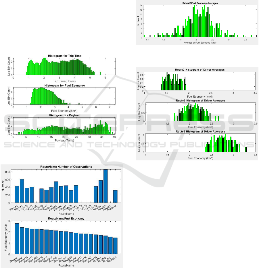
The available data included observations for 21
different routes, most of which were frequently
driven over the relevant period by a set of 331 drivers.
In order to investigate the impact of route
characteristics and driver behaviour, the available
data set was categorized per route. Figure 3 displays
the number of trips available per route as well as the
average fuel economy per route, sorted from highest
to lowest. It can be seen that the average fuel
economy per route varies by almost a factor of two
from the least to the most fuel efficient. Figure 4
displays the histogram of average fuel economy per
driver across all routes. For drivers the spread of
averages is even wider than for routes; this may
however partly be as a result of route inclination and
payload variations.
Figure 2: Histograms for trip times, fuel economy and
payload.
Figure 3: Number of trips and average fuel economy per
route.
In Figure 5 we display the driver average fuel
economy histograms for a few individual routes; it
can be seen that within a specific route the variation
in performance between drivers is not quite as big as
across all routes. The driver variations within the
same route are however sufficiently large to justify a
more accurate comparison between drivers, aimed at
quantifying the potential for fuel economy
improvement, should all drivers perform at the same
level.
Figure 4: Histogram of average fuel economy per driver for
all routes.
Figure 5: Histograms of average fuel economy per driver
for individual routes.
4 EXTRACTING EMPIRICAL
FUEL ECONOMY MODELS
In a previous article (Hoffman and Van der
Westhuizen, 2019) we described the extraction of
linear fuel economy regression models, as well as
nonlinear regression models based on the following
formula:


i
= 

0
+ 

1



+ 

3



+ 

2n-1



(1)
where


i
is the estimated fuel economy value for observation
i
X
ni
are the values of input variables for observation i
NCTA 2019 - 11th International Conference on Neural Computation Theory and Applications
382



0 -


2n
are the estimates of the population regression
slopes and exponents as indicated above.
In this paper we expand this work by also
extracting neural network models using identical input
and target variables, and comparing the results
produced by the different models. The first type of
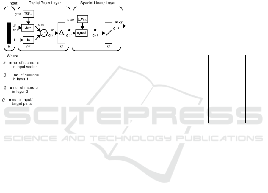
neural model is a generalized regression neural
network (GRNN) that is a variation on radial basis
function networks. The network architecture is
illustrated in Figure 6 below.
Figure 6: Architecture of the GRNN network.
This network uses a spread parameter to regularize
the input-output relationship; the value of spread is the
distance between the centre of a radial basis function
and the points where its magnitude has decreased by a
factor of 2. Larger values of spread therefore result in
smoother input-ouput mappings. We experimented
with GRNN models where the value of spread was
allowed to vary between 1 and 2024 in steps by a factor
of 2. The number of radial basis functions equalled the
number of training observations.
The second type of neural network that was used is
the multilayer perceptron, using a single hidden layer
with sigmoid transfer functions and a linear output
layer. In this case the number of hidden nodes is used
to regularize the input-output mapping: larger numbers
of hidden nodes provide more accurate fitting within
the training set, but may lead to overfitting, resulting in
lack of generalization ability in the test set, while a
smaller number of hidden nodes will result in less good
fits for the training set but more closely matching
goodness of fit for the test set. In our case we allowed
the number of hidden nodes to vary between 2 and 32.
We extracted models using all four modeling
techniques (linear regression, nonlinear regression,
GRNN and MLP NN) from the earliest 70% of all
observations, and predicted fuel economy for the
remaining 30% of observations. In order to compare
our results with results from previous research, we first
extracted models using driver, route and payload
factors as inputs. Input factors were selected by
ranking potential inputs based on absolute value of
linear correlations between inputs and fuel economy.
Table 2 provides the Pearson correlation coefficients
between a list of available input factors and fuel
economy. We only included input factors with a
correlation coefficient of at least 0.1 with the model
target. Once a ranked input factor has been selected,
we only considered additional factors that had a
correlation with already selected factors of less than
0.4, as the use of several higly correlated inputs results
in unstable model parameters.
Table 2: Correlation coefficients between fuel economy and
potential explanatory variables.
Inputs
Corr
Inputs
Corr
Max Speed
-0,133
Payload
-0,174
Speeding Time
-0,044
Elev Gain (m)
-0,627
Max Brake
0,018
Elev Lost (m)
0,465
Excessive Brake Time
-0,010
Max Slope Asc
-0,581
Excessive Accel Time
-0,016
Max Slope Desc
0,333
Max RPM
-0,378
Ave Slope Asc
-0,594
Excessive RPM Time
-0,014
Ave Slope Desc
0,443
Excessive Idle Time
0,026
Elev Gain (m/km)
-0,611
Standing Time
0,061
Elev Lost (m/km)
0,385
The list of model parameters selected on this basis
included Elevtion Gain, Max RPM, Payload and Max
Speed. Elevation Lost and some other factors were not
selected based on their high correlations with Elevation
Gain, that was selected first as it had the highest
absolute correlation with fuel economy.
The regression coefficients for the linear and
nonlinear regression models are displayed in Table 2 to
Table 4 below. For the nonlinear regression models
both the input factor coefficients and exponents are
given; for the linear models the exponents are always
1 as indicated. It can be seen that the relationships
between some inputs factors and fuel economy is
significantly nonlinear, as some exponents deviate
substantially from a value of 1.
Figure 7 and Figure 8 displays scatterplots of
Target vs Output for the regression and neural models
respectively. Based on the scatterplots the model fits
for the test sets appear to be very similar to that for
the training sets, which indicates that the models have
good generalization capability. It can also be seen
that the neural models provide a superior fit of output
to target compared with the regression models, while
the GR neural network seem to be slightly superior to
the MLP network. These observations will be
confirmed using correlation analysis.
Neural Models for Benchmarking of Truck Driver Fuel Economy Performance
383

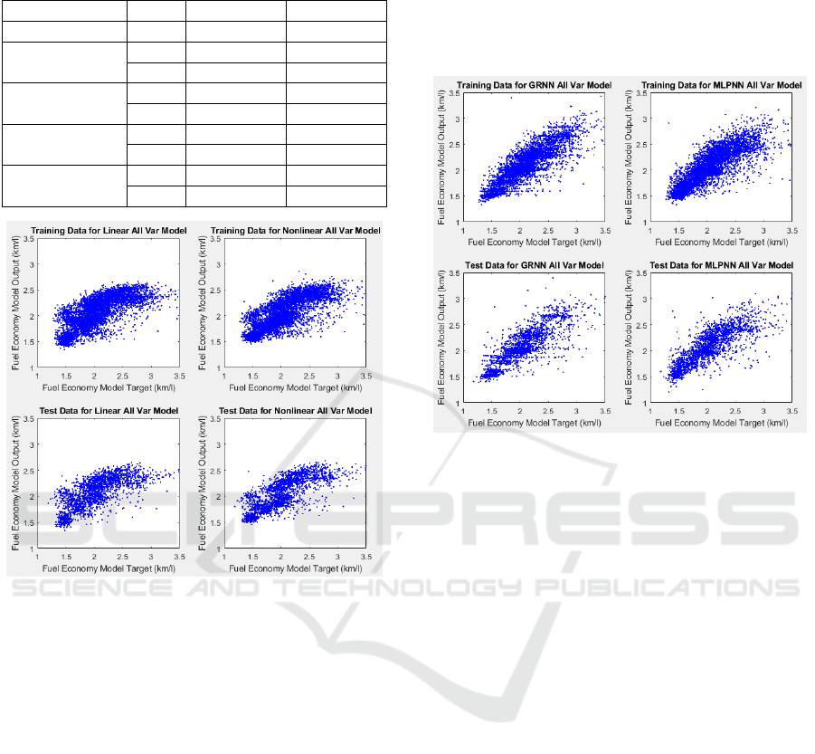
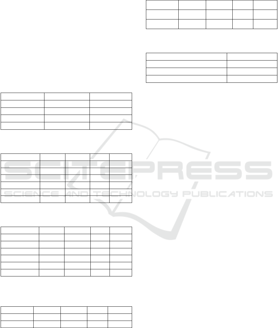
Table 3: Regression coefficients for general fuel economy
models.
Input Factor
Linear
Nonlinear
Constant
3,279
4,292
Max Speed
Coeff
0,006
0,007
Exp
1,000
0,945
Max RPM
Coeff
-0,001
-0,001
Exp
1,000
0,933
Payload
Coeff
-0,008
-0,101
Exp
1,000
0,514
Elevation Gain
Coeff
0,000
-0,136
Exp
1,000
0,348
Figure 7: Scatterplots for linear and nonlinear regression
Targets and Outputs.
More insight into nature of the various modelling
techniques is obtained by constructing input-output
graphs where one input is varied across its entire
range of values, while the remaining variables are
kept constant at their average values. As we created
the outputs using artificial inputs values, it is not
possible to display corresponding target values. We
constructed such graphs for the four model types, and
repeated this for different levels of regularization
applied to the neural models to observe the impact of
changing the spread parameter and the number of
hidden nodes. In the Figure 9 and Figure 10 below
we display the relationship between Elevation Gain
as input and the modelled Fuel Economy as output for
different levels of regularization applied to the neural
models.
It can be seen that all models display a similar
trend in the modelled relationship. When low levels
of regularization are applied to the neural models,
they tend to display extreme variations in the output,
which is indicative of overfitting. When the level of
regularization is increased, most of this behaviour
disappears, and the relationships are much closer to
those for the regression models. Similar results are
obtained when using Payload as input variable, as
displayed in Figure 11 and Figure 12.
Figure 8: Scatterplots for GRNN and MLP neural network
Targets and Outputs.
We subsequently extracted models that only used
inputs not impacted by driver behaviour; regression
coefficients for these models are displayed in Table 4
below. To assess driver impact on performance, we
extracted both a driver behavioural model, that
utilizes behavioural variables like Maximum RPM,
Speeding Time and Maximum Speed as inputs
(regression coefficients displayed in Table 5), as well
as a driverID model, that uses driver identity as input.
To model the impact of driver identity we defined
driver dummy variable inputs (one variable per driver
that assumes the value of one when the respective
driver is present and zero otherwise). A positive
driver ID regression model coefficient indicates
above average performance while a negative model
coefficient indicates below average performance. We
then proceeded to extract both driver models using
the residuals of the route inclication and payload
models as targets. For the driverID model we thus
obtain regression model coefficients that provide a
direct indication of driver performance, compensated
for the impact of route and payload. Comparison
between the two sets of driver ID model coefficients
before and after correcting for non-driver factors will
provide a clear indication of the impact of model
correction.
NCTA 2019 - 11th International Conference on Neural Computation Theory and Applications
384

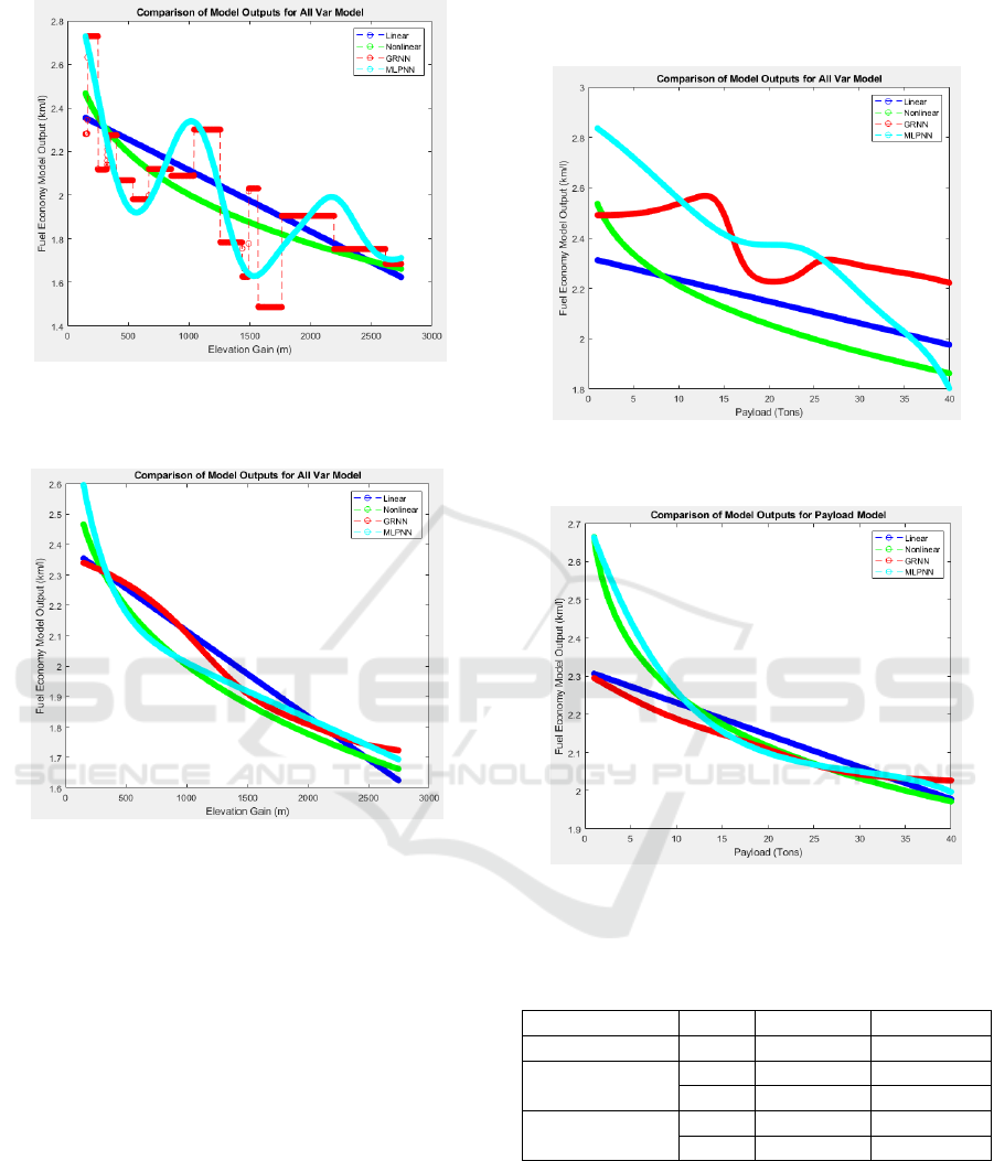
Figure 9: Elevation Gain vs Fuel Economy for all four
model types, using low levels of regularization for neural
models.
Figure 10: Elevation Gain vs Fuel Economy for all four
model types, using high levels of regularization for neural
models.
In order to evaluate model accuracy, we
calculated the correlations between model outputs
and target variables both for the training and test sets,
as displayed in Table 6 to Table 9 below. It can be
seen that the models that include driver, route and
payload inputs have the biggest correlations between
output and target, as would be expected. Most of the
correlation obtained in the training set is retained in
the test set, indicating that the observed relationships
between fuel economy and the respective explanatory
variables are strong and consistent. It can also be seen
that the nonlinear regression models perform slightly
superior to the linear regression models, while the
neural models outperform the regression models, both
for the general, the route & payload and the driver
models. The driver behavioural model, that uses Max
RPM, Max Brake and Max Speed as inputs, perform
slightly better than the driver ID model, that uses
driver identity as input.
Figure 11: Payload vs Fuel Economy for all four model
types, using low levels of regularization for neural models.
Figure 12: Payload vs Fuel Economy for all four model
types, using high levels of regularization for neural models.
Table 4: Regression coefficients for route and payload
models.
Input Factor
Linear
Nonlinear
Constant
2,707
4,540
Payload
Coeff
-0,012
-0,104
Exp
1,000
0,568
Elevation Gain
Coeff
0,000
-0,407
Exp
1,000
0,243
We investigated the consistency in driver
performance over time by correlating both the
uncompensated and compensated driver fuel
economies between the training and test sets. In
Table 10 below it can be seen that the consistency in
driver performance is increased by compensating for
the impact of route inclination and payload, as the
correlation between training and test set performance
Neural Models for Benchmarking of Truck Driver Fuel Economy Performance
385

is higher for compensated compared to
uncompensated performance. This confirms that
factors like route inclination and payload add
variability to driver performance measures that is
unrelated to actual driver performance. It is
furthermore observed that, after also compensating
for driver identify, the correlation of residual driver
performance between the training and test sets is
almost zero. This is to be expected as most of the
driver impact is now present in the driver model
output, with the remaining model residual fuel
economy being mostly noise.
Table 5: Linear regression coefficients for driver fuel
economy models (both uncompensated and compensated
for route and payload factors).
Input Factor
Uncompensated
Compensated
Const
4,702
-0,205
Max Speed
-0,001
0,001
Max RPM
-0,012
-0,009
Max Brake
0,019
-0,014
Table 6: Correlation coefficients between fuel economy
model outputs and targets for the training set.
Inputs
LinRegr
NonLinR
GRNN
MLPNN
All Var
0,695
0,721
0,856
0,800
Route
0,627
0,660
0,740
0,735
Payload
0,174
0,184
0,221
0,257
Route&Payload
0,671
0,705
0,814
0,783
DriverBeh
0,381
0,381
0,392
0,400
DriverID
0,357
-
0,300
0,327
Table 7: Correlation coefficients between fuel economy
model outputs and targets for the test set.
Inputs
LinRegr
NonLinRe
GRNN
MLPNN
All Var
0,592
0,655
0,763
0,741
Route
0,607
0,636
0,710
0,706
Payload
0,180
0,202
0,240
0,282
Route&Payload
0,640
0,678
0,768
0,744
DriverBeh
0,139
0,159
0,315
0,341
DriverID
0,121
-
0,127
0,148
Table 8: Training set correlation coefficients between
outputs and targets for models trained on the route and
payload residual fuel economy.
Inputs
LinRegr
NonLinR
GRNN
MLPNN
DriverBeh
0,263
0,262
0,271
0,277
DriverID
0,435
0,067
0,368
0,414
Table 9: Test set correlation coefficients between outputs
and targets for models trained on the route & payload
residual fuel economy.
Inputs
LinRegr
NonLinR
GRNN
MLPNN
DriverBeh
0,024
0,044
0,173
0,200
DriverID
0,134
0,033
0,112
0,131
Table 10: Correlations between driver fuel economy
performance measured over the training and test sets.
Fuel Economy Measure
Train vs Test Corr
Uncompensated
0,292
Route&Cargo Compensated
0,326
Driver,Route&Cargo Compensated
0,012
5 ESTIMATING MODEL
COMPENSATION IMPACT ON
DRIVER PERFORMANCE
MEASUREMENTS
One of our stated objectives is to measure driver
performance more consistently by compensating for
those factors over which the driver has no control. We
therefore calculated a compensated fuel economy
figure for each trip by subtracting the route & cargo
fuel economy model output from the original fuel
economy, and then adding the population average
fuel economy to this residual to obtain a fuel economy
figure that is mostly attributed to driver behaviour:
   
  
(2)
We expect variations in driving performance to be
reduced after compensating for the impact of route
and payload. To verify if this is the case we
calculated the standard deviation of uncompensated
driver fuel economy averages over all drivers, and
obtained a figure of 0.192 km/l. The compensated
driver fuel economy in equation 2 above was used to
calculate compensated driver averages. The standard
deviation of compensated driver averages was then
calculated as 0.158 km/l, which is indeed somewhat
lower than the figure before compensation.
Figure 13 displays histograms of the compensated
fuel economy using both the linear and nonlinear
route and payload models. When compared against
the uncompensated histogram the distributions have
clearly changed. In Figure 14 we compare
uncompensated versus route and cargo compensated
fuel economy histograms for a sample of drivers. The
change in distribution is clearly visible; in cases
NCTA 2019 - 11th International Conference on Neural Computation Theory and Applications
386

where the average did not change much, as for driver
923, the spread became narrower as expected, due to
removal of the impact of varying route inclinations
and payloads.
Figure 13: Histograms for route and cargo compensated
fuel economy.
To investigate the relationships between
uncompensated and compensated driver performance
measures, we calculated correlations between driver
fuel economy averages and the linear regression
model coefficients of the Driver ID based models.
Table 11 below displays the correlations between the
coefficients of both the uncompensated and route &
payload compensated Driver ID models, versus the
uncompensated and compensated fuel economies, as
observed over both the training and test sets. The
correlation between the uncompensated fuel
economy and uncompensated driver ID model
coefficients is almost 1 for the training set as
expected, as the model coefficients were extracted
from this data. For the test set it is still significantly
positive, confirming that driver ID explains a
significant fraction of observed fuel economy. We
also observe a large positive correlation between the
compensated driver ID model coefficients and
compensated fuel economy over the training set.
In contrast the correlations between the route
compensated Driver ID model coefficients and
uncompensated fuel economy are negative for both
the training and test sets; this indicates significant
differences between driver performance before and
after eliminating the impact of route inclination and
payload. It is confirmed by the fact that the route &
payload compensated fuel economy is also negatively
correlated with the uncompensated Driver ID model
coefficients for both the training and test sets. The
correlation of -0.729 between driver ID regression
coefficients before and after compensation confirms
how drastically driver performance assessment is
changed by the model correction. This is a very
important result, as it provides evidence for the
acceptance of our hypothesis that driver performance
measures are drastically impacted by the presence of
factors that are not identical for all drivers and not
within the driver’s control.
Figure 14: Comparison of uncompensated and route and
cargo compensated fuel economy histograms for different
drivers.
Table 11: Correlations between driver average fuel
economy and Driver ID based model coefficients.
Driver Fuel Economy
Coeff
Uncomp
Coeff Route
Comp
Uncompensated Train
0,976
-0,594
Uncompensated Test
0,243
-0,066
Route & Payload Comp Train
-0,581
0,525
Route & Payload Comp Test
-0,124
0,082
Driver & Route Comp Train
0,014
0,000
Driver & Route Comp Test
-0,383
0,536
DriverID Coeff Route Comp
-0,729
1
As a further confirmation of these results we
calculate correlations between average driver fuel
economy performance before and after
compensation. Table 12 indicates that driver
performance before and after route and payload
compensation is negatively correlated. The fact that
this is almost equally strong for the training and test
sets provides evidence that it is not as a result of
model overfitting. We furthermore observe that when
also removing the impact of driver ID the remaining
Neural Models for Benchmarking of Truck Driver Fuel Economy Performance
387

correlation for the training set is almost zero, as the
remaining model error will now have little
resemblance to the original fuel economy. A small
positive correlation remains for the test set as the
models could not capture all variations present in the
data; this is also to be expected as not all factors
impacting fuel economy are present in the model (e.g.
wind speed and traffic conditions).
Table 12: Correlations between compensated and
uncompensated driver fuel economy performance.
Variable
Train
Test
Route&Cargo Compensated
-0,598
-0,554
Driver,Route&Cargo Compensated
0,007
0,240
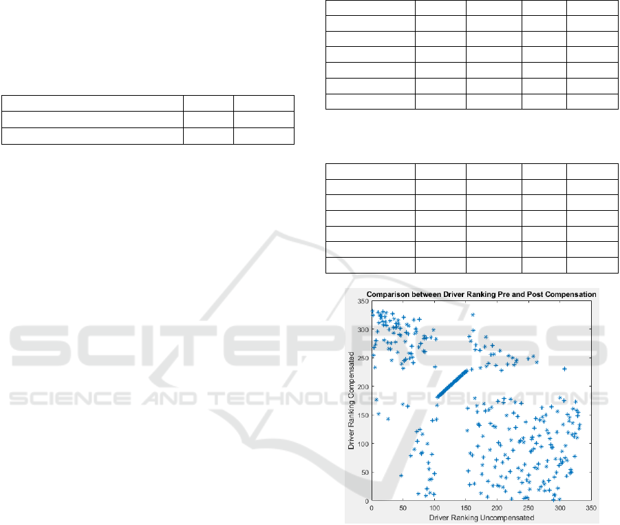
To quantify the degree to which driver
performance measures are impacted by model
compensation we calculated each driver’s ranking
compared to other drivers, firstly based on
uncompensated and secondly based on compensated
performance averages. For each driver the difference
in ranking position was determined before and after
model compensation; this change in ranking was
normalized by division through the total number of
drivers. The average absolute change in ranking
differences was then calculated over all drivers to
obtain an overall figure of the degree to which
ranking was impacted by performance compensation,
as indicated in equation 3 below:
  









(3)
where N is the total number of drivers.
For random changes to all driver rankings this
figure will be 0.5; for no ranking changes it will be
zero. To verify the consistency in driver performance
over time, we first calculated the relative change in
ranking between the training and test sets for both the
uncompensated and compensated fuel economies.
We obtained a relative ranking change of 0.27; this
indicates that performance does change over time, but
that it is not entirely random, with some level of
consistency. We then proceeded to compare the
ranking of driver performances between the case with
no compensation and the case after model
compensation. Table 13 and Table 14 displays the
relative ranking changes for different compensation
models for the training and test sets. It can be seen
that the change in driver ranking before and after
compensation is bigger than the difference of 0.27
observed between the training and test sets; this
indicates that, over and above changes in
performance over time, the model based
compensation results in a significant difference in
driver ranking.
Table 13: Average relative change in driver performance
ranking before and after compensation for the training set.
Inputs
LinRegr
NonLinR
GRNN
MLPNN
All Var
0,468
0,468
0,447
0,456
Route
0,477
0,469
0,465
0,466
Payload
0,493
0,489
0,495
0,494
Route&Payload
0,479
0,471
0,472
0,473
DriverBeh
0,460
0,459
0,482
0,458
DriverID
0,343
0,494
0,500
0,411
Table 14: Average relative change in driver performance
ranking before and after compensation for the test set.
Inputs
LinRegr
NonLinR
GRNN
MLPNN
All Var
0,471
0,468
0,462
0,462
Route
0,483
0,472
0,471
0,467
Payload
0,493
0,486
0,493
0,493
Route&Payload
0,482
0,464
0,473
0,475
DriverBeh
0,470
0,467
0,477
0,472
DriverID
0,414
0,495
0,499
0,445
Figure 15: Comparison between driver ranking before and
after compensating for route and cargo.
These results are confirmed by the scatterplot of
driver rankings before and after compensation as
displayed in Figure 15. The series of drivers that
seem to have retained the same ranking before and
after (straight line in the middle of the graph) are
drivers with no trips in the test set and to whom we
allocated average performance; they therefore
assumed sequential positions in the ranking list.
As a last measure of the impact of model
compensation we calculated the fraction of drivers for
whom performance relative to the population average
changed from positive to negative or vice versa after
NCTA 2019 - 11th International Conference on Neural Computation Theory and Applications
388

compensation. If performance before and after model
compensation is unrelated (e.g. random performance
changes) the total fraction of changes should be 0.5.
Table 15 displays the fraction of drivers with reversed
relative performance. We observe that for the route
& cargo model compensations the relative changes
are the biggest. For the driver models the fraction of
changes approach 0.5, because the residues from
these models are largely unrelated to driver identity
and would therefore appear to be random.
To compare the impact of the different models on
driver performance after correction, we calculated the
differences in average relative change in ranking
between the models. The comparison matrix in Table
16 provides evidence that all the models largely agree
in terms of the required changes in driver ranking, as
these differences are fairly close to zero (in those
cases where a model was compared against itself a
result of exactly zero was obtained). Lastly we
performed a similar comparison between route
models and payload models that used the same
modelling technique; these results appear in Table 17.
The differences are slightly larger than in the previous
case, as payload represents a smaller fraction of fuel
economy changes compared to route inclination and
is therefore less effective when used on its own.
Table 15: Fraction of drivers with reverse in relative
performance before and after compensation.
Inputs
LinRegr
NonLinR
GRNN
MLPNN
All Var
0,565
0,565
0,529
0,511
Route
0,577
0,565
0,544
0,532
Payload
0,601
0,592
0,592
0,583
Route&Payload
0,577
0,583
0,544
0,571
DriverBeh
0,565
0,553
0,577
0,562
DriverID
0,363
0,607
0,598
0,447
Table 16: Difference in average relative change in driver
performance ranking after compensation between on
different route and payload models.
Model Type
LinRegr
NonLinR
GRNN
MLPNN
LinRegress
0,000
0,070
0,091
0,078
NonLinRegr
0,070
0,000
0,109
0,095
GRNN
0,091
0,109
0,000
0,059
MLPNN
0,078
0,095
0,059
0,000
Table 17: Difference in average relative change in driver
performance ranking after compensation based on different
route vs payload models.
LinRegress
0,082
NonLinRegress
0,123
GRNN
0,100
MLPNN
0,121
6 CONCLUSIONS AND FUTURE
WORK
In this paper we derived models for truck fuel
economy using four different modelling techniques.
We proved that neural models outperform linear and
nonlinear regression models, regardless of the set of
input factors that are used, and that both radial basis
and MLP networks produced satisfactory results. We
also demonstrated that selecting the width of the
radial basis functions or the number of hidden layer
nodes can be used to obtain the required level of
accuracy and generalization ability.
The point of departure of our research was a
hypothesis that factors beyond the control of a truck
driver has a significant impact on fuel economy
performance measures. The results reported in this
paper provides conclusive evidence that the
hypothesis can be accepted. Firstly, we found that
factors like route inclination and payload explain a
significant fraction of total observed fuel economy
deviations. Secondly we observed that variations
between averages of driver performance are reduced
after compensating for route and payload. Thirdly we
found that there is more consistency between driver
performance in the training and test sets after
compensating for route and payload than before. In
the fourth place we proved that average driver
performance measured before and after compensating
for route and payload are negatively correlated. In the
fifth place we observed large changes in driver
performance ranking after compensation, and lastly
we found that the fuel economy performance of the
majority of drivers, relative to the population average,
changes in sign after compensating for route and
payload.
The default measure currently used for driver fuel
performance is the observed average over all
completed trips. The new performance measure that
we propose, to replace the default measure of average
over all completed trips, is to use the residual of the
model that predicts fuel economy in terms of route
inclinations and payload. The population average for
fuel economy is then added to this residual to obtain
a realistic fuel economy figure for each driver.
Future work will involve the inclusion of additional
input factors not related to driver behaviour, like wind
speed and traffic conditions, as factors to be
compensated for, as well as the use of more
sophisticated neural network techniques, e.g. using
clustering techniques to determine the optimal
number of radial basis functions.
Neural Models for Benchmarking of Truck Driver Fuel Economy Performance
389

REFERENCES
Anon., 2014. Stopping the flow of illegal black gold.
Transport World Africa, June, p. Vol. 12 No. 3.
Bennett, I. Greenwood, C., 1995. HDM-4 Fuel
Consumption Modelling, Preliminary Draft Report to
the International Study of Highway Development and
Management Tools, Birmingham: University of
Birmingham.
Biggs, D., 1988. ARFCOM - Models For Estimating Light
to Heavy Vehicle Fuel Consumption, Research Report
ARR 152, Nunawading: Australian Road Research
Board.
Delgado, O., Clark, N. Thompson, G., 2011. Modeling
Transit Bus Fuel Consumption on the Basis of Cycle
Properties. Journal of the Air & Waste Management
Association, pp. 443 - 452.
Elnaz Siami-Irdemoosa, S. R. D., 2015. Prediction of fuel
consumption of mining dump trucks: A neural networks
approach. Applied Energy 151, p. 77–84.
Gong, L., Morikawa, T., Yamamoto, T. Sato, H., 2014.
Deriving Personal Trip Data from GPS Data: A
Literature Review on the Existing Methodologies.
Beijing, China, s.n.
Hassanean S.H. Jassim, W. L. T. O., 2018. Assessing
energy consumption and carbon dioxide emissions of
off-highway trucks in earthwork operations: An
artificial neural network model. Journal of Cleaner
Production 198, pp. 364-380.
Havenga, J., 2013. 10th Annual State of Logistics Survey
for South Africa, ISBN number: 978-0-7988-5616-4, p.
9., Stellenbosch, South Africa: s.n.
Hoffman, A. J., 2010. The use of technology for trade
corridor management in Africa. Sandton,
Johannesburg, South Africa, s.n.
Hoffman, A. J., Van der Westhuizen, M., 2014. An
Investigation into the Economics of Fuel Management
in the Freight Logistics Industry. Qingdao, PRC, s.n.
Hoffman, A. J. , Van der Westhuizen, M., 2019. An
empirical model for the assessment of truck driver fuel
economy. Auckland, New Zeeland, IEEE, p. to be
published.
Hoffman, A. , Van der Westhuizen, M., 2019. Empirical
model for truck route fuel economy. IEEE Intelligent
Transportation Systems Conference, p. Submitted for
publication.
Jian-Da Wu, J.-C. L., 2012. A forecasting system for car
fuel consumption using a radial basis function neural
network. Expert Systems with Applications Vol 39, p.
1883–1888.
Naidoo, J., 2013. Transport White Paper: The South
African Cross-Border Industry, THRIP Research
Report, Potchefstroom, South Africa: North-West
University.
Perrottaa, F. et al., 2019. Verification of the HDM-4 fuel
consumption model using a Big data approach: A UK
case study. Transportation Research Part D, pp. 109 -
118.
Rakha, J. , Wang, H., 2017. Fuel consumption model for
heavy duty diesel trucks: Model development and
testing. Transportation Research Part D, pp. 127 - 141.
United States Environmental Protection Agency, 2019.
Sources of Greenhouse Gas Emissions. [Online]
Available at: https://www.epa.gov/ghgemissions/
sources-greenhouse-gas-emissions
United States Environmental Protection Agency, 2019.
Transportation and Climate Change. [Online]
Available at: https://www.epa.gov/transportation-air-
pollution-and-climate-change/carbon-pollution-
transportation
Weille, J. d., 1966. Quantification of Road User Savings.
World Bank Occasional Papers No. 2, World Bank,
Washington D.C..
Zhigang Xu, T. W. S. E. X. Z., 2018. Modeling
Relationship between Truck Fuel Consumption and
Driving Behavior Using Data from Internet of Vehicles.
Computer-Aided Civil and Infrastructure Engineering
Vol 33, p. 209–219.
NCTA 2019 - 11th International Conference on Neural Computation Theory and Applications
390