A Regression-like Classiﬁcation System for Geometric Semantic Genetic

Programming

Illya Bakurov

, Mauro Castelli

, Francesco Fontanella

and Leonardo Vanneschi

NOVA Information Management School (NOVA IMS), Universidade Nova de Lisboa,

Campus de Campolide, 1070-312, Lisbon, Portugal

Department of Electrical Engineering and Information, Universit

a degli Studi di Cassino e del Lazio Meridionale,

03043, Cassino, Italy

Keywords:

Classiﬁcation, Regression, Geometric Semantic Genetic Programming.

Abstract:

Geometric Semantic Genetic Programming (GSGP) is a recent variant of Genetic Programming, that is gain-

ing popularity thanks to its ability to induce a unimodal error surface for any supervised learning problem.

Nevertheless, so far GSGP has been applied to the real world basically only on regression problems. This

paper represents an attempt to apply GSGP to real world classiﬁcation problems. Taking inspiration from Per-

ceptron neural networks, we represent class labels as numbers and we use an activation function to constraint

the output of the solutions in a given range of possible values. In this way, the classiﬁcation problem is turned

into a regression one, and traditional GSGP can be used. In this work, we focus on binary classiﬁcation;

logistic constraining outputs in [0,1] is used as an activation function and the class labels are transformed into

0 and 1. The use of the logistic activation function helps to improve the generalization ability of the system.

The presented results are encouraging: our regression-based classiﬁcation system was able to obtain results

that are better than, or comparable to, the ones of a set of competitor machine learning methods, on a rather

rich set of real-life test problems.

1 INTRODUCTION

Geometric Semantic Genetic Program-

ming (GSGP) (Moraglio et al., 2012) is a recent

development of Genetic Programming (GP) (Koza,

1992). GSGP uses particular genetic operators,

called Geometric Semantic Operators (GSOs) and it

has gained noteworthy popularity among researchers

in the last few years. This popularity is probably

because GSOs can induce a unimodal error surface

(i.e., with no locally optimal solutions) for any

supervised learning problem. This property bestows

a remarkable optimization power on GSGP. Further-

more, in several references (see for instance (Castelli

et al., 2015a)), it was shown that, in some particular

circumstances, GSOs are also able to limit over-

ﬁtting. Thanks to these important properties, and

also to a very efﬁcient implementation presented

in (Castelli et al., 2015a), GSGP was successful in

several different real-life applications in recent years

(a rather complete summary of the applications is

reported in (Vanneschi et al., 2014)).

However, looking at the different applications

that have been developed with GSGP, it is possi-

ble to notice a clear trend: those applications are

mainly regression and forecasting problems. In other

words, almost no relevant results showing success-

ful applications of GSGP on classiﬁcation problems

were presented. This does not happen by chance:

even though in the contribution that originally in-

troduced GSGP (Moraglio et al., 2012) a version

of GSOs for classiﬁcation was presented, that version

of the operators is not very easy to use. More specif-

ically, those operators assume that GSGP is evolving

individuals that are classiﬁcation rules. Even though

systems evolving rules, like decision trees, using GP

have been presented so far, this is not the most typical

use of GP. GP individuals are, typically, mathematical

functions of the inputs, returning as output numbers.

As such, GP is naturally more prone to be used for

regression than for classiﬁcation.

In this paper, we intend to ﬁll this gap, proposing

a GSGP-based approach for classiﬁcation for the ﬁrst

time, where individuals are numeric expressions, as

is usual in GP. The approach is straightforward and

inspired by the output layer of Artiﬁcial Neural Net-

works (ANNs), where an activation function is ap-

plied to the output. Similarly to ANNs, a logistic ac-

Bakurov, I., Castelli, M., Fontanella, F. and Vanneschi, L.

A Regression-like Classiﬁcation System for Geometric Semantic Genetic Programming.

DOI: 10.5220/0008052900400048

In Proceedings of the 11th International Joint Conference on Computational Intelligence (IJCCI 2019), pages 40-48

ISBN: 978-989-758-384-1

tivation is applied to the output of a GSGP individual,

and compared to the target of a binary classiﬁcation,

appropriately transformed into binary values (with 0

representing one class label, and 1 representing the

other). It is worth noticing that, since the problem is

“de facto” transformed into a regression and the lo-

gistic function is increasing monotonically, the prop-

erty of GSOs of inducing a unimodal error surface is

maintained. Despite its simplicity, we think that, if

successful, this idea may have a signiﬁcant impact,

paving the way for new GSGP contributions for real-

life classiﬁcation problems.

The paper is organized as follows: in Section 2,

we describe GSGP; Section 3 presents our idea of a

regression-like classiﬁcation system based on GSGP;

Section 4.3 contains our experimental study. More

speciﬁcally, in the ﬁrst part of this section, we present

experiments aimed at tuning two important system

parameters, while in the second part we present an ex-

perimental comparison of the proposed approach with

Support Vector Machines, one of the most popular

and powerful classiﬁcation algorithms. The compari-

son is made on 10 complex real-life datasets. Finally,

Section 5 concludes the work, and presents ideas for

future investigation.

2 GEOMETRIC SEMANTIC

GENETIC PROGRAMMING

Let X = {

−→

,...,

−→

} be the set of input data (train-

ing instances, observations or ﬁtness cases) of a sym-

bolic regression problem, and

−→

t = [t

,...,t

] the

vector of the respective expected output or target val-

ues (in other words, for each i = 1,2,...,n, t

is the

expected output corresponding to input

−→

). A GP

individual (or program) P can be seen as a function

that, for each input vector

−→

returns the scalar value

−→

). Following (Moraglio et al., 2012), we call se-

mantics of P the vector

−→

= [P(

−→

),P(

−→

),...,P(

−→

)].

This vector can be represented as a point in an n-

dimensional space, that we call semantic space. Re-

mark that the target vector

−→

t itself is a point in the

semantic space.

As explained above, GSGP is a variant of GP

where the traditional crossover and mutation are re-

placed by new operators called Geometric Semantic

Operators (GSOs). The objective of GSOs is to de-

ﬁne modiﬁcations on the syntax of GP individuals that

have a precise effect on their semantics. More in par-

ticular, as schematically shown in Figure 1, GSOs are:

• Geometric Semantic Crossover. This operator

generates only one offspring, whose semantics

stands in the line joining the semantics of the two

parents in the semantic space.

• Geometric Semantic Mutation. With this opera-

tor, by mutating an individual i, we obtain another

individual j such that the semantics of j stands

inside a ball of a given predetermined radius, cen-

tered in the semantics of i.

One of the reasons why GSOs became so popular in

the GP community (Castelli et al., 2015d; Castelli

et al., 2013; Castelli et al., 2015c; Ruberto et al.,

2014; Castelli et al., 2015e; Castelli et al., 2016b;

Castelli et al., 2015b; Vanneschi et al., 2017; Bakurov

et al., 2018; Bartashevich et al., 2018) is related to

the fact that GSOs induce an unimodal error surface

(on training data) for any supervised learning prob-

lem, where ﬁtness is calculated using an error mea-

sure between outputs and targets. In other words, us-

ing GSOs the error surface on training data is guaran-

teed to not have any locally optimal solution. This

property holds, for instance, for any regression or

classiﬁcation problem, independently of how big and

how complex data are (Vanneschi et al., 2014; Castelli

et al., 2016a). The deﬁnitions of the GSOs are, as

given in (Moraglio et al., 2012), respectively:

Geometric Semantic Crossover (GSC). Given

two parent functions T

: R

→ R, the geomet-

ric semantic crossover returns the real function

= (T

· T

) + ((1 − T

) · T

), where T

is a ran-

dom real function whose output values range in the

interval [0,1].

Geometric Semantic Mutation (GSM). Given a par-

ent function T : R

→ R, the geometric semantic mu-

tation with mutation step ms returns the real function

= T + ms · (T

− T

), where T

and T

are ran-

dom real functions.

Even though this is not in the original deﬁnition

of GSM, later contributions (Castelli et al., 2015a;

Castelli et al., 2014) have clearly shown that limiting

the codomain of T

and T

in a predeﬁned interval

(for instace [0,1], as is done for T

in GSC) helps

improving the generalization ability of GSGP. As

in several previous works (Vanneschi et al., 2014;

Castelli et al., 2015a), here we constrain the outputs

of T

, T

and T

by wrapping them in a logistic

function. Only the deﬁnitions of the GSOs for

symbolic regression problems are given here, since

they are the only ones used in this work. For the

deﬁnition of GSOs for other domains, the reader is

referred to (Moraglio et al., 2012). Figure 1 shows a

graphical representation of the mapping between the

syntactic and semantic space given by the GSOs.

Using these operators, the semantics of the off-

spring is completely deﬁned by the semantics of the

A Regression-like Classiﬁcation System for Geometric Semantic Genetic Programming

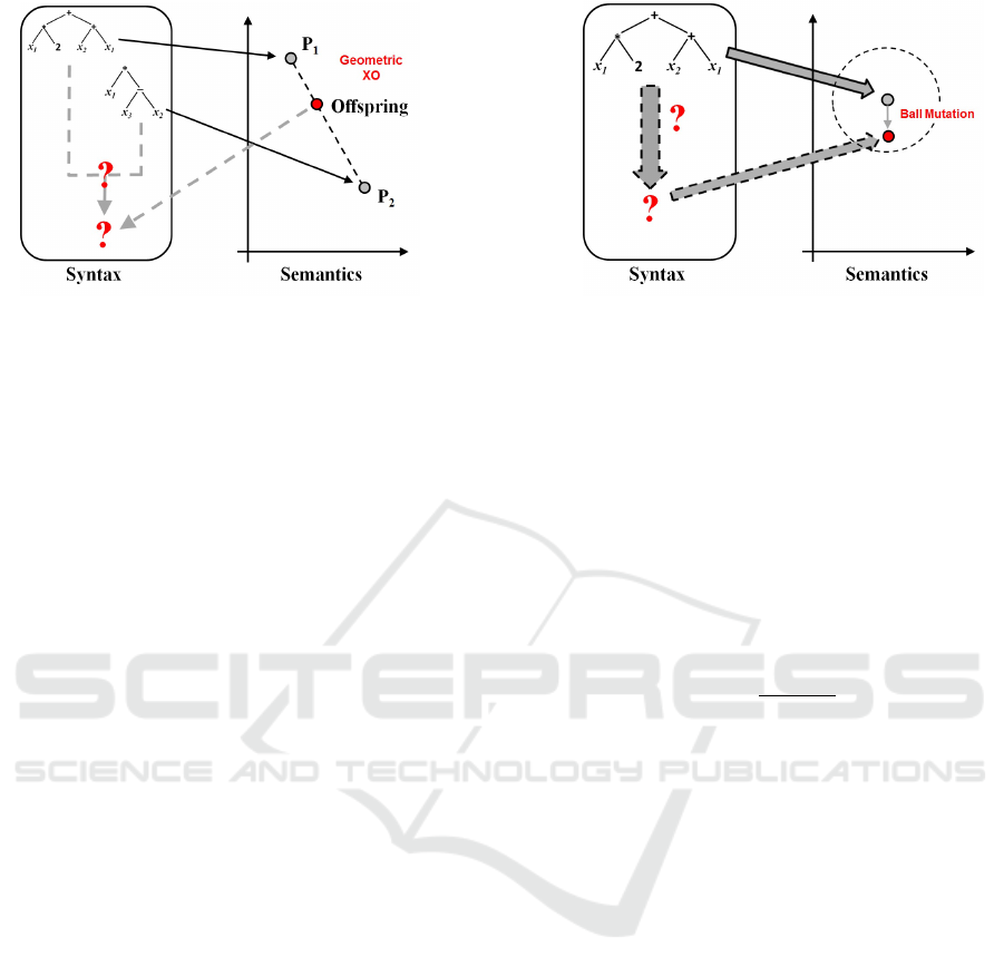
(a) (b)

Figure 1: Geometric semantic crossover (plot (a)) (respectively geometric semantic mutation (plot (b))) performs a trans-

formation on the syntax of the individual that corresponds to geometric crossover (respectively geometric mutation) on the

semantic space. In this ﬁgure, the unrealistic case of a bidimensional semantic space is considered, for simplicity.

parents: the semantics of an offspring produced by

GSC will lie on the segment between the semantics

of both parents (geometric crossover), while GSM de-

ﬁnes a mutation such that the semantics of the off-

spring lies within the ball of radius ms that surrounds

the semantics of the parent (geometric mutation).

As reported in (Moraglio et al., 2012), the prop-

erty of GSOs of inducing a unimodal error surface

has a price. The price, in this case, is that GSOs al-

ways generate larger offspring than the parents, and

this entails a rapid growth of the size of the individ-

uals in the population. To counteract this problem,

in (Castelli et al., 2015a) an implementation of GSOs

was proposed that makes GSGP not only usable in

practice, but also signiﬁcantly faster than standard GP.

This is possible by means of a smart representation

of GP individuals, that allows us not to store their

genotypes during the evolution. This is the imple-

mentation used here. Even though this implementa-

tion is efﬁcient, it does not solve the problem of the

size of the ﬁnal model: the genotype of the ﬁnal so-

lution returned by GSGP can be reconstructed, but it

is so large that it is practically impossible to under-

stand. This turns GSGP into a “black-box” system,

as many other popular machine learning systems are,

including deep neural networks.

3 REGRESSION-LIKE

CLASSIFICATION WITH GSGP

In this work, we use symbolic regression GSOs

to solve binary classiﬁcation problems. The used

method is inspired by the functioning of the Percep-

tron neural network (Vanneschi and Castelli, 2019).

The two class labels that characterize the problem are

transformed into two numeric values. The values 0

and 1 have been used in this work. In this way, the

classiﬁcation problem can be imagined as a regres-

sion problem, containing only 0 and 1 as possible tar-

get values. The output of a GP individual P is given

as input to an activation function, and the ﬁtness of P

is the Root Mean Square Error (RMSE) between the

output of the activation function and the binary tar-

get. As customary in Perceptrons, we have used the

logistic activation function:

L(x) =

1 + e

−αx

(1)

This function has two asymptotes, respectively in 0

and 1, that are the target values we have used. Us-

ing this activation function should help us to improve

the generalization ability of the system, since faith-

fully approximating the target values 0 and 1 entails

a separation of data belonging to different classes. In

other words, the evolutionary process automatically

pushes towards the generation of GP individuals that

return large positive values for observations labeled

with 1, and large negative values for observations la-

beled with 0. At the same time, a good individual

should not return small values for any of the obser-

vations, since those small outputs would immediately

give a deteriorating contribution to the error.

This effect of data separation can be tuned by

modifying constant α in Equation (1). In order to have

a visual intuition of this, Figure 2 shows two different

logistic functions, one with α = 1 (plot (a)), and the

other with α = 0.1 (plot (b)).

From this ﬁgure, it is possible to see that, in order

to obtain the same approximation of an output value

equal to 1 (respectively 0), when α = 0.1 the output

has to be larger (respectively smaller), compared to

the case α = 1. So, for the same value of the er-

ror, data belonging to different classes are better sep-

arated for smaller values of α. On the other hand, of

ECTA 2019 - 11th International Conference on Evolutionary Computation Theory and Applications

(a) α = 1 (b) α = 0.1

Figure 2: Graphical representation of logistic functions (Equation (1)) with two different values of the α parameter.

Plot (a): α = 1; Plot (b): α = 0.1.

course, using small values of α also has a drawback:

given a preﬁxed value of the training error ε, ﬁnding

individuals with an error equal to ε will be computa-

tionally harder for smaller values of α. All this con-

sidered, ﬁnding the appropriate value of α, represent-

ing a good compromise between generalization abil-

ity and computational cost, is a challenge and various

preliminary tuning experiments have been needed, in

order to obtain the value used here. Once a model op-

timizing the RMSE on training data has been found,

it can be used for generalization on unseen data, sim-

ply using a threshold equal to zero on the output: ob-

servations with positive outputs will be predicted as

belonging to one of the two classes, while the other

observations will be categorized in the other class.

4 EXPERIMENTAL STUDY

4.1 Test Problems

In order to assess the effectiveness of the proposed ap-

proach, we considered ten binary classiﬁcation prob-

lems, which present different characteristics in terms

of the number of attributes and instances. The related

datasets are publicly available on the UCI (Dua and

Karra Taniskidou, 2017) and openML (Vanschoren

et al., 2013) repositories. Table 1 reports, for each one

of these problems, the number of input features (vari-

ables) and data instances (observations) in the respec-

tive datasets and the repository from which the data

have been downloaded.

Since for each feature the range of values may

vary widely, data was normalized by using the Z-

normalization method: for each feature f

, we ﬁrst

computed the mean µ

and the standard deviation σ

on the training set, then we applied the following

transformation:

i j

− µ

where x

i j

is the value of the i-th feature from the j −th

Table 1: Description of the benchmark problems. For each

dataset, the number of features (independent variables), the

number of instances (observations) that were reported.

Dataset #Features #Instances Repository

Fertility 9 100 openML

Hill 100 1212 openML

Ilpd 10 579 openML

Liver 6 345 UCI

Mammo 5 830 UCI

Musk 166 476 UCI

Qsar 41 1055 UCI

Retinopathy 19 1151 UCI

Spam 57 3037 UCI

Spect 22 266 UCI

Table 2: Parametrization used in the experiments.

Parameters Values

Population size 500

# generations 2000

Tree initialization Ramped Half-and-Half,

maximum depth 6

Crossover rate 0.0

Mutation rate 1.0

Function set +,−,∗, and protected /

Terminal set Input variables, random con-

stants

tournament size 4

Elitism Best individual always sur-

vives

# random trees 500

sample (both from the training or the test set) and z

i j

is the corresponding normalized value.

4.2 Experimental Settings

During the experimental study, we performed two sets

of experiments. In the ﬁrst set we investigated the

classiﬁcation performances of the proposed approach

as function of α and R, which represent the steepness

of the curve and width of the range for the random

constants in the terminal set, respectively. In the sec-

A Regression-like Classiﬁcation System for Geometric Semantic Genetic Programming

ond set of experiments, instead, we compared the re-

sults achieved by our GSGP-based binary classiﬁca-

tion system with those of an SVM classiﬁer.

For all the considered test problems, 30 indepen-

dent runs of each studied system were executed. For

each problem, the related dataset was randomly split

into an equally sized and statistically independent

training and test set. The RMSE (see Section 3) on

the training set was used to compute the ﬁtness of

each individual, whereas the error rate on the test set

was used to assess the classiﬁcation performance on

unseen data of the best individual found at the end

of each run. All the results reported in the following

were computed averaging these classiﬁcation results.

As for the parameters, we performed some prelimi-

nary trials to set them. These parameters were used

for all the experiments described below and are re-

ported in Table 2.

4.3 Experimental Results

As mentioned in previously, we performed two sets

of experiments. The ﬁrst to ﬁnd the best values for

the parameters α and R, and the second to compare

our results with those achieved by an SVM classiﬁer.

Both sets of experiments are described as follows.

In the ﬁrst set of experiments, we investigated how

the values ofα and R affect the classiﬁcation perfor-

mance of our system since both values affect the ﬁnal

output of the GP individuals. The former, which rep-

resents the limits of the range of the random constants

[−R,+R], affects the values the random constants of

the terminal set can assume, thus affecting the input

values given as input to the GP trees. As for α, as

mentioned in Section 3, it affects the separation of

samples belonging to different classes, with small α

values ensuring a better separation than larger ones

(see Figure 2). For this reason, we performed a facto-

rial experiment to investigate the relationship between

these two parameters. More speciﬁcally, we consid-

ered the following sets of parameters:

= {0.0001,0.001,0.01,0.05,0.1,0.2, 0.5}

= {1,2,5,10,20,50}

As for the remaining parameters, we used those

shown in Table 2. The plots in Figures 3 and 4 show

the test error as a function of the R for the different

α values tested. From the Figures it can be noted

Given an individual GP individual I representing the

function f

: R

→ R, where R

is the feature space, the test

sample x is labeled as belonging to the class 0 if f (x) > 0,

to the class 1 otherwise. In practice, the logistic function

is only used for training the system. This because in any

binary classiﬁcation problem, the classiﬁer must provide as

output a class label (0 or 1), instead of a numerical value.

that for all the considered datasets, too low α values

achieve the worse performance. In particular, the val-

ues 0.0001 and 0.001 achieve the worst performance,

while for most of the datasets, the value 0.01 per-

forms worse than the higher values. Moreover, it is

worth noting that for these three values the ”perfor-

mance ranking”, the performance differences among

these values, is kept for all the datasets and for all the

R values. These results prove that too low α values do

not improve the ”data separation” effect mentioned in

Section 3. This is most probably because these val-

ues produce too ﬂat curves (similar to straight lines

with a low slope). In practice, these α values produce

similar output values for a large range of input values

returned by the GP individuals, thus reducing the se-

lective pressure of the evolutionary process. It is also

worth noting that the curves for these values exhibit a

high variability with respect to R, even if there is no

monotonic trend, that would prove that higher (lower)

R values perform better. As for the remaining α val-

ues (0.05,0.1,0.2,0.5) from the plots, it can be noted

that:

(i) in most of the cases they achieve similar results;

(ii) even when their performances are signiﬁcantly

different, the related curves tend to be over-

lapped;

(iii) on several datasets (see for example Musk in

Figure 3(c) or Spam in Figure 4(c)) the value 0.5

tends to perform better than the smaller values.

Maybe a better explanation for these results is that

these α values allow better differentiation between

samples belonging to different classes, with the posi-

tive (negative) ones labeled as 1 (0) and correctly clas-

siﬁed by GP individuals yielding positive (negative)

outputs. In fact, for an individual I the error for a

given sample x is computed as

(L( f

(x)) −l

)

(2)

where f

(x) is the function encoded by I, L the

(logistic) activation function (see Equation 1) and l

the label of x (0 or 1). Then, according to the above

equation, the effect of higher α values is twofold:

they allow reducing the RMSE for correct classiﬁca-

tion even when f

returns small values and increasing

the RMSE even for misclassiﬁcations characterized

by small values. In practice, those higher α values

better reward/penalize correctly/incorrectly classiﬁed

instances.

To better explain this concept, we drew the logistic

function for these values (Figure 5) and we also com-

puted the output values of the logistic functions for

these remaining α for some samples. From the table it

is worth noting that for small f (x) output values (see

ECTA 2019 - 11th International Conference on Evolutionary Computation Theory and Applications

(a) Fertility (b) Hill

(e) Mammo (f) Musk

Figure 3: Test error as a function of the limits of the range of the random constants [−R,+R] for the ﬁrst six datasets of

Table 1.

for examples the samples 1 and 3), L with α = 0.05 re-

turns similar values both for correctly (sample #1) and

incorrectly classiﬁed (sample #3) samples, whereas

with α = 0.5 L returns quite different values for these

samples. Similar considerations can be done for the

other samples. For example, for the misclassiﬁed

sample #8, with f

(x) = −11.2, L returns 0.41 with

α = 0.05, whereas it returns 0.00 with α = 0.5.

4.4 Comparison with SVMs

In order to test the effectiveness of the proposed ap-

proach, we compared its results with those achieved

by a Support Vector Machine (SVM). Support Vec-

tor Machines (SVMs) are supervised learning meth-

Table 3: Output values of the logistic functions for some

samples, where f

(x) is the output value of a generic GP

individual I. Rows in bold represent misclassiﬁed samples.

# l

(x) (L( f

(x)) −l

)

(Eq. (2))

0.05 0.1 0.2 0.5

1 0 -1.6 0.23 0.21 0.18 0.10

2 0 -16.5 0.093 0.026 0.001 6.8e-8

3 0 1.2 0.27 0.28 0.31 0.42

4 0 7.2 0.35 0.45 0.65 0.95

5 1 1.4 0.23 0.22 0.19 0.11

6 1 3.5 0.21 0.17 0.11 0.02

7 1 -2 0.28 0.30 0.36 0.53

8 1 -11.2 0.41 0.57 0.82 0.99

9 1 6.1 0.18 0.12 0.05 2.04e-3

A Regression-like Classiﬁcation System for Geometric Semantic Genetic Programming

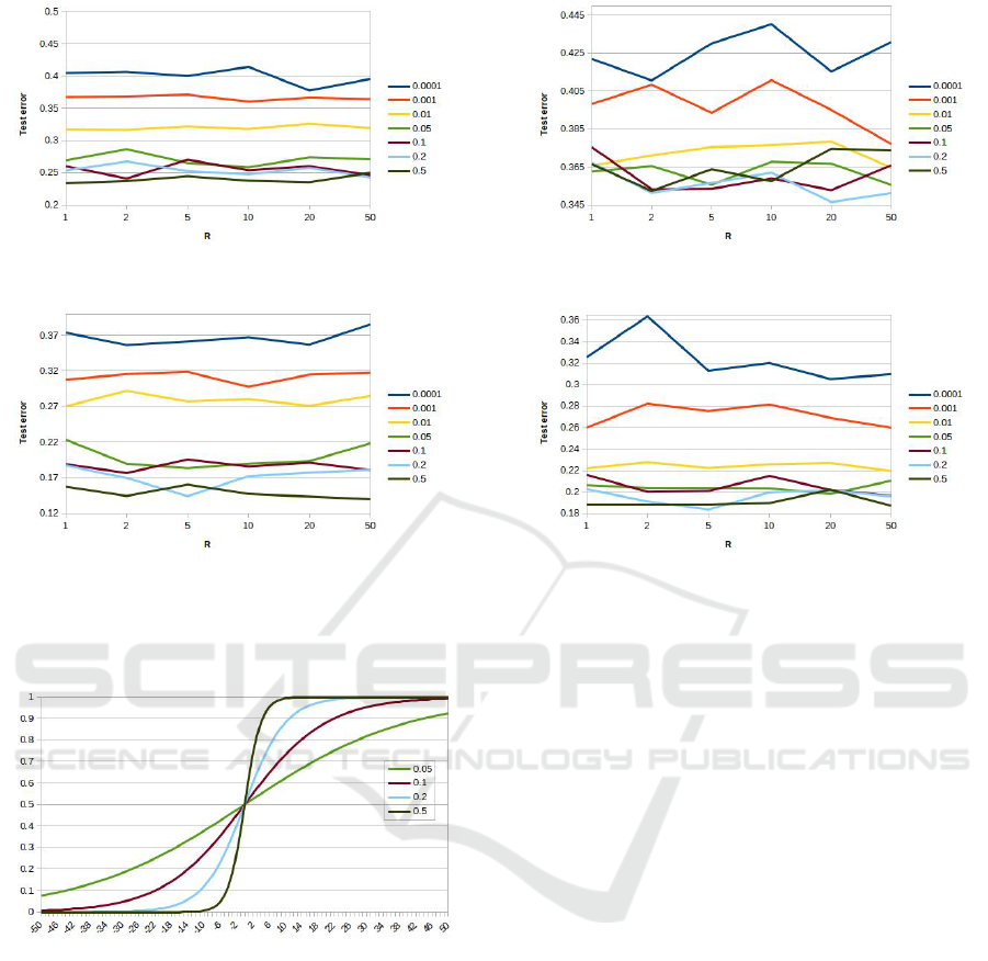
(a) Qsar (b) Retinopathy

Figure 4: Test error as a function of the limits of the range of the random constants [−R,+R] for the last four datasets of Table

Figure 5: The logistic functions for the α values: 0.05, 0.1,

0.2 and 0.5.

ods that are based on the concept of decision planes,

which linearly separates, in the feature space, objects

belonging to the different classes (Cortes and Vapnik,

1995). Intuitively, given two classes to be discrimi-

nated in a given feature space, a good separation is

achieved by the hyperplanes that have the largest dis-

tance to the nearest training points belonging to dif-

ferent classes; in general, the larger the margin, the

lower the generalization error of the classiﬁer. While

the basic idea of the SVM applies to linear classiﬁers,

they can be easily adapted to non-linear classiﬁca-

tion tasks by using the so called ”kernel trick”, which

implies the mapping of the original features into a

higher dimensional feature space. Differently from

other classiﬁer schemes, whose learning usually im-

plies stochastic and suboptimal gradient descent pro-

cedures, e.g., NN and DT, given a training set, the

SVM learning optimization problem can be solved by

using quadratic programming algorithms which pro-

vide exact solutions. SVMs have shown to be ef-

fective in solving many real world applications like

handwriting recognition, text categorization and im-

age classiﬁcation (Byun and Lee, 2002).

As suggested by (Lin and Lin, 2003; Keerthi and Lin,

2003), we chose the radial basis function (RBF) as

kernel in our experiments:

K(x, y) = e

−γkx−yk

where x and y are two generic samples in the feature

space.

As for the implementation, we used that provided

by the LIBSVM public domain software (Chang and

Lin, 2011). Moreover, to perform a fair comparison

with the GSGP, for each considered problem, we per-

formed 30 runs. As mentioned before, SVMs are de-

terministic, i.e. for a given training set the algorithm

always returns the same set of support vectors. For

this reason, to get averaged results on unseen data, for

each run the data was randomly shufﬂed and split into

a training and a test set, equally sized. The results

reported in the following have been averaged on the

ECTA 2019 - 11th International Conference on Evolutionary Computation Theory and Applications

accuracy obtained on the 30 generated test sets.

To statistically validate the comparison results,

we performed the non-parametric Wilcoxon rank-sum

test. The comparison results are shown in Table 4,

which also shows the p-value for the Wilcoxon test.

From the table it can be observed that on eight of the

ten considered problems, our GSGP-based classiﬁer

outperforms the SVM, while as for the remaining two

(Fertility and Mammo), the differences are not statis-

tically signiﬁcant (p-value > 0.05). Moreover, from

the table it can be also noted that in most of the cases

performance differences increase with the number of

features. This seems to suggest that the evolutionary

search process implemented by our approach is able

to: (i) effectively identify the features that better dis-

criminate samples belonging to different classes; (ii)

effectively ﬁnd the functions (expressions) of these

features that characterize the classes of the problem

at hand.

5 CONCLUSIONS AND FUTURE

WORK

A new classiﬁcation approach based on Geometric

Semantic Genetic Programming (GSGP) was pre-

sented in this paper. Despite the simplicity of the idea,

the presented results showed that this approach was

able to outperform Support Vector Machines (SVMs)

on 8 different complex real-life problems, returning

comparable results on the remaining 2 test problems.

These results encourages us to pursue the idea, and we

believe that this work could pave the way to a set of

applicative successes, comparable with the ones that

GSGP has obtained on regression and forecasting in

recent years (Vanneschi et al., 2014).

An important part of our current work is an at-

tempt of extending the proposed approach to multi-

Table 4: Comparison results (accuracy, expressed in per-

centage) between the proposed approach and the SVM clas-

siﬁer. Rows in bold highlight problems with no statistical

signiﬁcant differences.

Dataset SVM GSGP p-value

Fertility 87.07 87.40 0.7024

Hill 51.00 61.28 1.73e-6

Ilpd 71.16 74.44 1.90e-6

Liver 58.84 64.73 2.34e-6

Mammo 80.23 80.29 0.7584

Musk1 61.08 75.00 2.34e-6

Qsar 67.01 76.63 7.68e-6

Retinopathy 59.40 65.35 3.52e-6

Spam 69.86 86.01 1.73e-6

Spect 79.27 81.65 2.20e-3

class classiﬁcation. Our objective is, if possible, to be

able to solve, with success, complex multi-class clas-

siﬁcation tasks, maintaining the simplicity of the idea

presented here. Furthermore, in the future, we plan

to integrate the proposed approach with local search

strategies and with regularization algorithms, in order

to further stress, possibly at the same time, its opti-

mization power on training data, and its generaliza-

tion ability. Inheriting ideas from SVMs, like maxi-

mum separation hyperplane and kernel trick, is also

a possibility that we are considering to extend the

work. Last but not least, we are planning to imple-

ment a parallel and distributed version of the system,

with highly heterogeneous populations. In this way,

different variants of the algorithm could be executed

in parallel, like different parameter settings, different

representations for the solutions, different activation

functions and different ﬁtness functions, just to men-

tion a few.

ACKNOWLEDGMENTS

This work was supported by national funds through

FCT (Fundac¸

ao para a Ci

encia e a Tecnologia)

under project DSAIPA/DS/0022/2018 (GADgET)

and project PTDC/CCI-INF/29168/2017 (BINDER).

Mauro Castelli acknowledges the ﬁnancial support

from the Slovenian Research Agency (research core

funding No. P5-0410).

REFERENCES

Bakurov, I., Vanneschi, L., Castelli, M., and Fontanella, F.

(2018). Edda-v2–an improvement of the evolution-

ary demes despeciation algorithm. In International

Conference on Parallel Problem Solving from Nature,

pages 185–196. Springer.

Bartashevich, P., Bakurov, I., Mostaghim, S., and Van-

neschi, L. (2018). Pso-based search rules for aerial

swarms against unexplored vector ﬁelds via genetic

programming. In International Conference on Par-

allel Problem Solving from Nature, pages 41–53.

Springer.

Byun, H. and Lee, S.-W. (2002). Applications of support

vector machines for pattern recognition: A survey. In

Proceedings of the First International Workshop on

Pattern Recognition with Support Vector Machines,

pages 213–236, London, UK. Springer-Verlag.

Castelli, M., Castaldi, D., Giordani, I., Silva, S., Vanneschi,

L., Archetti, F., and Maccagnola, D. (2013). An ef-

ﬁcient implementation of geometric semantic genetic

programming for anticoagulation level prediction in

pharmacogenetics. In Portuguese Conference on Arti-

ﬁcial Intelligence, pages 78–89. Springer.

A Regression-like Classiﬁcation System for Geometric Semantic Genetic Programming

Castelli, M., Silva, S., and Vanneschi, L. (2015a). A

c++ framework for geometric semantic genetic pro-

gramming. Genetic Programming and Evolvable Ma-

chines, 16(1):73–81.

Castelli, M., Trujillo, L., and Vanneschi, L. (2015b). Energy

consumption forecasting using semantic-based ge-

netic programming with local search optimizer. Com-

putational intelligence and neuroscience, 2015:57.

Castelli, M., Trujillo, L., Vanneschi, L., Silva, S., et al.

(2015c). Geometric semantic genetic programming

with local search. In Proceedings of the 2015 An-

nual Conference on Genetic and Evolutionary Com-

putation, pages 999–1006. ACM.

Castelli, M., Vanneschi, L., and De Felice, M. (2015d).

Forecasting short-term electricity consumption using

a semantics-based genetic programming framework:

The south italy case. Energy Economics, 47:37–41.

Castelli, M., Vanneschi, L., Manzoni, L., and Popovi

c, A.

(2016a). Semantic genetic programming for fast and

accurate data knowledge discovery. Swarm and Evo-

lutionary Computation, 26:1–7.

Castelli, M., Vanneschi, L., and Popovi

c, A. (2015e). Pre-

dicting burned areas of forest ﬁres: an artiﬁcial intel-

ligence approach. Fire ecology, 11(1):106–118.

Castelli, M., Vanneschi, L., and Popovi

c, A. (2016b). Pa-

rameter evaluation of geometric semantic genetic pro-

gramming in pharmacokinetics. International Journal

of Bio-Inspired Computation, 8(1):42–50.

Castelli, M., Vanneschi, L., and Silva, S. (2014). Prediction

of the uniﬁed parkinson’s disease rating scale assess-

ment using a genetic programming system with ge-

ometric semantic genetic operators. Expert Systems

with Applications, 41(10):4608–4616.

Chang, C.-C. and Lin, C.-J. (2011). LIBSVM: A library for

support vector machines. ACM Transactions on Intel-

ligent Systems and Technology, 2:27:1–27:27. Soft-

ware available at http://www.csie.ntu.edu.tw/

cjlin/libsvm.

Cortes, C. and Vapnik, V. (1995). Support-vector networks.

Machine Learning, 20(3):273–297.

Dua, D. and Karra Taniskidou, E. (2017). UCI machine

learning repository.

Keerthi, S. S. and Lin, C.-J. (2003). Asymptotic behaviors

of support vector machines with gaussian kernel. Neu-

ral Computation, 15(7):1667–1689.

Koza, J. R. (1992). Genetic Programming: On the Pro-

gramming of Computers by Means of Natural Selec-

tion. MIT Press, Cambridge, MA, USA.

Lin, H.-T. and Lin, C.-J. (2003). A study on sigmoid ker-

nels for svm and the training of non-psd kernels by

smo-type methods. Technical report, Department of

Computer Science, National Taiwan University.

Moraglio, A., Krawiec, K., and Johnson, C. (2012). Ge-

ometric semantic genetic programming. In Coello,

C., Cutello, V., Deb, K., Forrest, S., Nicosia, G., and

Pavone, M., editors, Parallel Problem Solving from

Nature - PPSN XII, volume 7491 of Lecture Notes in

Computer Science, pages 21–31. Springer Berlin Hei-

delberg.

Ruberto, S., Vanneschi, L., Castelli, M., and Silva, S.

(2014). Esagp–a semantic gp framework based on

alignment in the error space. In European Conference

on Genetic Programming, pages 150–161. Springer.

Vanneschi, L., Bakurov, I., and Castelli, M. (2017). An ini-

tialization technique for geometric semantic gp based

on demes evolution and despeciation. In Evolutionary

Computation (CEC), 2017 IEEE Congress on, pages

113–120. IEEE.

Vanneschi, L. and Castelli, M. (2019). Multilayer percep-

trons. In Ranganathan, S., Gribskov, M., Nakai, K.,

and Sch

onbach, C., editors, Encyclopedia of Bioinfor-

matics and Computational Biology, pages 612 – 620.

Academic Press, Oxford.

Vanneschi, L., Silva, S., Castelli, M., and Manzoni, L.

(2014). Geometric semantic genetic programming for

real life applications. In Genetic programming theory

and practice xi, pages 191–209. Springer.

Vanschoren, J., van Rijn, J. N., Bischl, B., and Torgo,

L. (2013). Openml: Networked science in machine

learning. SIGKDD Explorations, 15(2):49–60.

ECTA 2019 - 11th International Conference on Evolutionary Computation Theory and Applications