Application of Mixtures of Gaussians for Tracking Clusters in
Spatio-temporal Data
Benjamin Ertl
1
, J
¨
org Meyer
1
, Achim Streit
1
and Matthias Schneider
2
1
Steinbuch Centre for Computing (SCC), Karlsruhe Institute of Technology (KIT), Karlsruhe, Germany
2
Institute of Meteorology and Climate Research (IMK-ASF), Karlsruhe Institute of Technology (KIT), Karlsruhe, Germany
Keywords:
Machine Learning, Pattern Recognition, Clustering, Spatio-temporal Data, Mixtures of Gaussians,
Climate Research.
Abstract:
Clustering data based on their spatial and temporal similarity has become a research area with increasing pop-
ularity in the field of data mining and data analysis. However, most clustering models for spatio-temporal data
introduce additional complexity to the clustering process as well as scalability becomes a significant issue for
the analysis. This article proposes a data-driven approach for tracking clusters with changing properties over
time and space. The proposed method extracts cluster features based on Gaussian mixture models and tracks
their spatial and temporal changes without incorporating them into the clustering process. This approach al-
lows the application of different methods for comparing and tracking similar and changing cluster properties.
We provide verification and runtime analysis on a synthetic dataset and experimental evaluation on a clima-
tology dataset of satellite observations demonstrating a performant method to track clusters with changing
spatio-temporal features.
1 INTRODUCTION
With the increasing amount of spatio-temporal data
researchers across a wide variety of disciplines
are facing new challenges mining and analysing
datasets. Spatio-temporal data exhibit observations
across space and time for example gathered by large
sensor networks or satellites providing remote sensing
or satellite imagery data. Spatio-temporal clustering
is an active research area analysing spatial and tem-
poral data at a higher level of abstraction by grouping
data points according to their similarity into meaning-
ful clusters (Trevor et al., 2009). Current approaches
leverage variations of well-known methods and algo-
rithms modified to operate on spatio-temporal data
(Maciag, 2017). In this context approaches have been
adapted for analysing trajectories and moving spatio-
temporal clusters (Li et al., 2004; Kalnis et al., 2005).
While current approaches often help to reveal and un-
derstand potential relationships many proposed meth-
ods lack the exploitation of available a priori knowl-
edge that might improve the output quality (Maimon,
2010). Additionally, current algorithms are often lim-
ited in detecting substructures in large datasets; es-
pecially when clusters are overlapping, for example
when observations are taken continuously at the same
locations, as it is often the case with spatio-temporal
data. In this paper we propose a data-driven ap-
proach of tracking clusters in spatio-temporal data.
Our approach is based on the Gaussian mixture model
to extract cluster properties that can be analysed for
changes over space and time. The concept is eval-
uated against synthetic data and real world climatol-
ogy data from satellite observations. We provide a
methodology based on well-known algorithms and an
interpretation of the algorithmic results in a spatio-
temporal context. Future possible extensions and
modifications to the applied algorithms will be dis-
cussed in the conclusion of the paper.
The remainder of the paper is organized as fol-
lows: Section 2 provides the background on the Gaus-
sian mixture model and the Bayesian Information Cri-
terion for model selection while Section 3 presents
the proposed concept in detail. Section 4 compares
our proposed concept to related work and Section
5 presents the evaluation and exemplification of the
concept in the area of climate research. At the end
in Section 6 we give a discussion on the results while
Section 7 provides the conclusions and outlooks.
All datasets together with the code for
Ertl, B., Meyer, J., Streit, A. and Schneider, M.
Application of Mixtures of Gaussians for Tracking Clusters in Spatio-temporal Data.
DOI: 10.5220/0007949700450054
In Proceedings of the 11th International Joint Conference on Knowledge Discovery, Knowledge Engineering and Knowledge Management (IC3K 2019), pages 45-54
ISBN: 978-989-758-382-7
Copyright
c
 2019 by SCITEPRESS – Science and Technology Publications, Lda. All rights reserved
45

this paper are publicly available online at
https://github.com/bertl4398/kdir2019.
2 PRELIMINARIES
This section shortly recalls the essential basics
for this paper: the Gaussian mixture model and
the Expectation-Maximization algorithm for fitting
Mixture-of-Gaussian models to the given data to-
gether with the Bayesian Information Criterion for
model evaluation.
2.1 Gaussian Mixture Model
Finite mixtures of distributions provide a sound
mathematical-based approach for statistical mod-
elling of a wide variety of random phenomena
(McLachlan and Basford, 1988; McLachlan and Peel,
2004). These probabilistic models consist of super-
position formed by linear combinations of basic dis-
tributions. By using a sufficient number of Gaussian
distributions with adjusted means and covariances as
well as adjusted contribution to the linear combina-
tion, any continuous density can be approximated to
arbitrary accuracy with few exceptions. A Gaussian
mixture model (GMM) can therefore be formulated
as following (Bishop, 2006)
p(x) =
K
∑
k=1
π
k
N (x|µ
k
, Σ
k
) (1)
with each Gaussian density components
N (x|µ
k
, Σ
k
) having its own mean µ
k
and covari-
ance Σ
k
. The parameters π
k
are called mixing
coefficients, satisfying the condition
K
∑
k=1
π
k
= 1 (2)
Using the maximum likelihood to set the values
for µ
k
, Σ
k
and π
k
, the logarithm of the likelihood func-
tion from (1) is given by
ln p(X|π, µ, Σ) =
N
∑
n=1
ln
(
K
∑
k=1
π
k
N (x|µ
k
, Σ
k
)
(3)
summing over N number of observations. Be-
cause of the summation over the number of clusters k
Equation (3) has no closed-form analytic solution but
can be estimated with the Expectation-Maximization
algorithm.
2.2 Expectation Maximization
The Expectation-Maximization (EM) algorithm finds
the local optimum for parameters in the likelihood
for models with latent variables from the given data
(Dempster et al., 1977).
For the Gaussian mixture model the algorithm first
initializes the means µ
k
, covariances Σ
k
and mixing
coefficients π
k
and evaluates the initial value of the
log likelihood. After initializing the parameters the
algorithm iterates over expectation and maximization
steps until convergence for maximizing the likelihood
function.
In the expectation step posterior probabilities for
each responsibility that the i-th data point x
i
belongs
to the k-th component of the mixture are computed as
follows.
p(z
k
= 1|x
i
) =
p(z
k
= 1)p(x
i
|z
k
= 1)
∑
k
p(z
k
= 1)p(x
i
|z
k
= 1)
(4)
Where z
k
is the k-th element of the binary random
variable z with
∑
k
z
k
= 1 and z
k
∈ 0, 1, specified in
terms of the mixing coefficients π
k
such that p(z
k
=
1) = π
k
.
In the maximization step the parameters µ
k
, Σ
k
and
π
k
can be re-estimated using the computed responsi-
bilities.
µ
k
=
∑
i
n
p(z
k
= 1|x
i
)x
i
o
∑
i
p(z
k
= 1|x
i
)
Σ
k
=
∑
i
n
p(z
k
= 1|x
i
)(x
i
− µ
k
)(x
i
− µ
k
)
T
o
∑
i
p(z
k
= 1|x
i
)
π
k
=
∑
i
p(z
k
= 1|x
i
)
N
(5)
If the convergence criterion is not satisfied the al-
gorithm returns to the expectation step.
2.3 Bayesian Information Criterion
Selecting the number of components in the Gaussian
mixture model can be done in an efficient way with
the Bayesian Information Criterion (BIC) (Chen and
Gopalakrishnan, 1998) penalizing the likelihood by
the number of clusters C
k
. The number of parameters
for each cluster is d +
1
2
d(d + 1) with data points x
i
∈
R
d
.
BIC(C
k
) =
k
∑
j=1
(
−
1
2
n
j
log|Σ
j
|
)
−Nk(d +
1
2
d(d +1))
(6)
KDIR 2019 - 11th International Conference on Knowledge Discovery and Information Retrieval
46

By selecting the Gaussian mixture model with the
lowest BIC we can ensure to choose the true num-
ber of clusters according to the intrinsic complex-
ity present in a particular dataset in the asymptotic
regime. This means, that the probability that BIC will
select the correct model approaches one with increas-
ing number of models up to infinity, but will tend to
choose models that might be to simple, because of the
penalty on complexity (Maimon, 2010).
3 PROPOSED MODEL
In this paper we propose a data-driven model to track
clusters and their changing properties over space
and time, based on the Gaussian mixture model and
Bayesian Information Criterion as introduced in the
previous Section 2. The model can be outlined in
four basic steps.
1. Splitting the Data in Spatial Regions of Interest:
This first step needs careful consideration if splitting
the data has a significant effect on the mixture compo-
nents by including or excluding certain observations
(”edge-effects”). Also splitting the data in spatial re-
gions of interest (ROI) might not always be applica-
ble, for example if all the clusters are tracked within
one spatial area.
However, if the nature of the dataset allows the
statistical evaluation and mitigation of edge-effects,
for example by assuming or proofing complete spa-
tial randomness (Diggle, 2013), and if the analysis is
conducted over multiple spatial areas, this step signif-
icantly increases the scalability of the model.
Each mixture model for any ROI can be computed
in parallel, which decreases the overall runtime, see
Section 5. Selection criteria for the size of the
ROI typically depends on domain knowledge or the
premise of the analysis.
2. Modelling the Observed Data in each ROI
with Mixtures of Gaussians: For each spatial re-
gion a range of Gaussian mixture component models
with different maximum number of mixture compo-
nents are fitted to the data. The model with the low-
est Bayesian Information Criterion score determines
the number of clusters for the most suitable mixture
model, as described in the preliminaries in Section 2.
An alternative approach to infer the number of
clusters of the most suited mixture model is the
variational Bayes approach (Attias, 1999). This
approach however requires additional fine tuning of
hyperparameters and introduces additional computa-
tional overhead.
3. Extracting Cluster Parameters for each
Gaussian Mixture Component: Following a data
summarization approach, we propose to extract the
ellipsoid properties of the multivariate Gaussian
distribution, the center and principal axes given
by the mean and length of the eigenvectors of the
covariance matrix as well as the polar angle of the
major axis, since theses properties most prominently
describe the underlying distribution. However,
different cluster properties can be selected according
to the nature of the data and the expected behaviour
of spatio-temporal changes of the clusters.
4. Comparison of Cluster Parameters for Spatio-
temporal Changes: The comparison can be done by
a range of suitable methods, which demonstrates the
flexibility of the proposed model. For the model eval-
uation and results in this paper, we used the DBSCAN
clustering algorithm (Ester et al., 1996) on the ex-
tracted cluster properties to find similar clusters and
account for spatio-temporal changes.
By comparing the extracted cluster parameters be-
tween clusters in different spatial regions over time
we can identify similar clusters and further review
these occurrences to investigate any underlying mo-
tion.
4 RELATED WORK
Using Gaussian mixture models for image match-
ing has been proposed in a continuous probabilistic
framework by Greenspan et al. (2001). Greenspan
et al. propose a transition of the image pixels to
coherent regions in feature space via Gaussian mix-
tures to apply a probabilistic measure of similarity be-
tween the Gaussian mixtures. To determine the num-
ber of mixture components Greenspan proposes the
minimum description length principle compared be-
tween cluster sizes ranging from three to six. Similar
images are identified by the Kullback–Leibler diver-
gence (Kullback, 1997) of their mixing components.
Compared to our approach we are not relying on the
Kullback–Leibler divergence measure to identify sim-
ilar mixing components, but extract cluster features
that can be further clustered for similarity with differ-
ent cluster algorithms.
A dynamic model-based clustering method for
spatio-temporal data with finite mixtures of Gaussians
with spatio-temporal varying mixing weights was pre-
sented by Paci and Finazzi (2018). In their work,
Application of Mixtures of Gaussians for Tracking Clusters in Spatio-temporal Data
47

Paci and Finazzi adjusted the mixing coefficients in
a way that similar observations at near space and time
points are assigned with similar cluster membership’s
probabilities. However, the model is only formulated
for the univariate case of observations and also the
Bayesian approach has a higher model bias then the
proposed model in this paper.
Jin et al. (2005a,b) proposed a clustering system
based on the Gaussian mixture model with indepen-
dent attributes within clusters. They modified the
EM-algorithm introduced in Section 2 to include the
clustering features of sub-clusters. Jin et al. use on
the one hand a grid-based method for cluster features
extraction and on the other hand the BIRCH clus-
tering algorithm (Zhang et al., 1996). In our pro-
posed model, we use the Gaussian mixture model for
data summarization and an additional clustering al-
gorithm to group similar cluster properties together.
The advantage of our approach is that we do not need
to modify the Expectation Maximization algorithm
and allow the application of different clustering algo-
rithms that might be better suited for data with outliers
or noise.
Providing a more formal definition of moving
clusters, Kalnis et al. (2005) present three algorithms
based on the DBSCAN clustering algorithm to iden-
tify moving clusters over a period of time. Moving
clusters are identified over consecutive time slices if
the ratio of their intersect density to their joint density
is greater or equal as a specified threshold. While al-
lowing to track clusters based on their densities over
time, the presented work by Kalnis does not pro-
vide the necessary means to monitor changing cluster
properties over space and time. Our approach does
not demand intersecting densities to identify mov-
ing clusters and is further able to identify reappearing
clusters and can track clusters with changing proper-
ties over space and time as well.
5 MODEL EVALUATION
In this section we evaluate or proposed model on a
synthetic dataset and a real dataset of satellite obser-
vations.
The synthetic dataset has been generated of simi-
lar size and structure as our real dataset, but with al-
ready known distributions in feature space. The spa-
tial points are generated from a N-conditioned Com-
plete Spatial Randomness (CSR) process (Diggle,
2013). A N-conditioned CSR process is defined as:
Given the total number of events N occurring within
an area A, the locations of the N events represent
Table 1: Dataset Descriptions.
Time steps Real data Synthetic data
# points # points
2014-02-12 154,031 160,001
2014-02-13 157,719 160,000
2014-02-14 167,473 160,000
2014-02-15 161,441 160,000
2014-02-16 155,187 160,000
2014-02-17 164,059 159,999
Total 959,910 960,000
Features {x, y} {ln(H
2
O), δD}
Spatial extent 162 clusters 162 20x20 boxes
an independent random sample of N locations where
each location is equally likely to be chosen as an
event (Rey and Anselin, 2007). The two dimensional
feature patterns are well separated isotropic Gaussian
blobs and assigned to k-means clustered spatial re-
gions. The spatial partitioning in the data generation
process (k-means clustered spatial regions) is differ-
ent from the spatial partitioning in the analysis (reg-
ular lattice) to better evaluate possible edge-effects.
The number of k-means clusters is equal to the num-
ber of spatial grid cells, 162, so that clusters and grid
cells have similar spatial extent, but some data points
at the cluster edges will be assigned to different grid
cells during the analysis.
The satellite observations have been gathered by
Metop-A and Metop-B satellites with the IASI (In-
frared Atmospheric Sounding Interferometer) instru-
ment (EUMETSAT, 2018). IASI measures in the in-
frared part of the electromagnetic spectrum at a hori-
zontal resolution of 12 km over a swath width of about
2,200 km, providing information on the vertical struc-
ture of the atmospheric temperature and humidity in
an unprecedented accuracy of 1 K and a vertical reso-
lution of 1 km. Compared to the synthetic data points,
the real observations are less dense due to different fil-
ters, missing observations and processing errors. Ide-
ally, we would have global coverage with no missing
data points and only variations in the distributions of
latitude and longitude of the satellite measurements
as in our synthetic dataset. Table 1 outlines the two
datasets, while a visualization of both datasets is pro-
vided in Figure 1 and 2. Additionally, all data is pro-
vided publicly available online.
We applied our proposed model described in
Section 3 on each of the six consecutive days in Table
1 as follows:
1. Splitting the Data in Spatial Regions of Interest:
We split the data into geospatial regions on a regular
grid with grid size of 20 x 20 degrees for longitude
KDIR 2019 - 11th International Conference on Knowledge Discovery and Information Retrieval
48

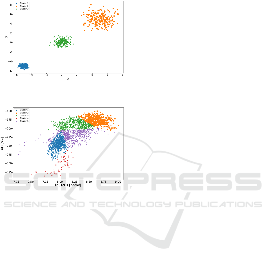
Figure 1: Feature distribution of a random grid cell for the
synthetic dataset. Markers and colors correspond to the
GMM clusters identified.
Figure 2: Feature distribution of a random grid cell for the
climatology dataset. Markers and colors correspond to the
GMM clusters identified.
180 degrees West to 180 degrees East and latitude
90 degrees South to 90 degrees North. The size of
the ROIs here is postulated by the domain expert to
conduct an analysis of far-reaching climatological
events. This step results into 162 ROIs, which we
impose on our real and synthetic dataset.
2. Modelling the Observed Data in each ROI with
Mixtures of Gaussians: For each spatial region we
fit multiple Gaussian mixture models with at least two
observations per cluster and a maximum number of
10 components. Each model is evaluated according
to its BIC score and the model with the lowest BIC
score is selected as the best model. The maximum
number of 10 components has been selected out of
multiple experimental runs, where we determined the
trade-off between searching for models with a higher
number of components and lower BIC scores and the
number of observations per cluster.
3. Extracting Cluster Parameters for each Gaus-
sian Mixture Component: For each Gaussian
mixture component identified in step 2, we extracted
the ellipsoid properties of the multivariate Gaussian
distribution, the center and principal axes given by
the mean and eigenvectors of the covariance matrix as
well as the angle of the major axis. More specifically
we extracted the major and minor axis length and the
axis angle in degrees for the bivariate contour where
95% of the probability falls.
4. Comparison of Cluster Parameters for Spatio-
temporal Changes: In the last step we used the DB-
SCAN algorithm with a maximum distance between
two samples E ps = 0.3 and the number of minimum
points MinPts = 2 in each Eps-neighbourhood. Each
Eps-neighbourhood is defined by the specified ra-
dius E ps and the number of minimum points MinPts
within E ps from a point under consideration, so that
this point can be identified as a core point. For further
details on the DBSCAN algorithm we refer to the pa-
per of Ester et al. (1996). Similar to step 2, the DB-
SCAN parameters have been assessed and evaluated
on the data through empirical analysis.
5.1 Verification
To verify our model we take a look at the feature dis-
tributions and the corresponding GMM clusters to-
gether with the identified groups of clusters by the
DBSCAN algorithm.
We can visualize the identified groups of cluster
by the DBSCAN algorithm by plotting the mean ellip-
soids of each DBSCAN cluster. Figure 3 and Figure 4
show the ellipses defined by the extracted properties,
the major and minor axis length and the axis angle in
degrees for the bivariate 95% contour. The number of
clusters for the synthetic dataset shown in Figure 3 in-
dicates three groups of similar clusters in accordance
with our initially defined three separated clusters for
each spatial region. A fourth group is dedicated to
DBSCAN outlier results.
For the real dataset we can see much more over-
lapping groups of clusters depicted in Figure 4, in to-
tal 250 groups including the dedicated outlier group.
This result is consistent with the feature distribution
in the dataset, exemplified in Figure 2, and will be
further discussed in the next subsection.
As exemplified by the feature distributions of a
random spatial grid cell in Figure 1 and 2, the GMM
clusters in the synthetic dataset in Figure 1 are iden-
tified as clearly separable as generated, although the
imposed spatial lattice is different from the initial spa-
tial k-means clustering in the generation process. We
can conclude that as stated in Section 3 the synthetic
dataset allows the statistical evaluation and mitigation
Application of Mixtures of Gaussians for Tracking Clusters in Spatio-temporal Data
49

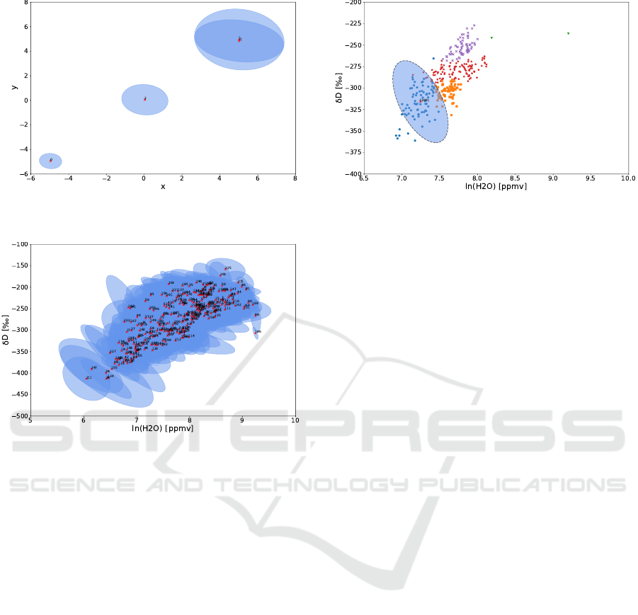
Figure 3: Mean ellipsoids of each DBSCAN cluster group
of clusters for the synthetic dataset.
Figure 4: Mean ellipsoids of each DBSCAN cluster group
of clusters for the climatology dataset.
of edge-effects. Data points that initially belong to a
different spatial region than our imposed lattice are
merely contributing to the feature distribution but do
not alter the distribution. The feature distribution in
the real dataset illustrated in Figure 2 do in contrast
not show any apparent separable clusters, however the
properties of the GMM clusters fitted to the data al-
lows to track moving clusters, emerging clusters and
cluster changes.
5.2 Application to Climate Research
Our real dataset consists of spectral data gathered
from Metop-A and Metop-B satellites that have been
processed for the water vapour H2O mixing ratio and
water isotopologue δD depletion for air masses at
5 km height with most sensitivity. The water iso-
topologue in question is HDO, which differs only
in the isotopic composition compared to H2O. Iso-
topologues of atmospheric water vapour can make a
significant contribution for a better understanding of
atmospheric water transport, because different water
transport pathways leave a distinctive isotopologue
fingerprint (Schneider et al., 2017).
Figure 5: Grid cell at latitude 50 degrees South to 30 de-
grees South and longitude 120 degrees East to 140 degrees
East at 2014-02-14. The ellipse visualizes the cluster prop-
erties of the moving cluster.
5.2.1 Tracking Moving Clusters
As an example of tracking moving clusters we are
looking at all GMM clusters that DBSCAN has as-
signed to the same group in neighbouring grid cells.
Here we identify moving clusters as clusters that ap-
pear in neighbouring grid cells with one day time
delay. This example has been selected for demon-
stration purpose, but the proposed method allows to
analyse similar clusters with different time lags and
paths across the imposed lattice as well. If two GMM
clusters are similar according to DBSCAN and one
is present in grid cell A at day 1 and present in grid
cell B, a neighbour grid cell to A, at day 2 we con-
clude that the cluster or cluster generating process
has moved from cell A to cell B. Our results show
multiple moving clusters according to the above def-
inition; specifically we could identify 105,616 occur-
rences that comply with the above definition of mov-
ing clusters. Figures 5 and 6 give one example of two
neighbouring grid cells with observations from 2014-
02-14 and 2014-02-15, at latitude 50 degrees South to
30 degrees South and longitude 120 degrees East to
140 degrees East and 140 degrees East to 160 degrees
East respectively. Both cells contain a specific clus-
ter that DBSCAN has assigned to the same group and
which is highlighted with the corresponding ellipses.
The presented result has been selected as a rep-
resentative example for detecting moving clusters be-
tween spatial regions. The clusters identified in Fig-
ure 5 and Figure 6 show close similarities and allow
additional visual verification. However, the proposed
method allows also to track clusters with varying clus-
ter properties, which might not be immediately appar-
ent.
Our proposed model is not limited to the defini-
tion of moving clusters used in this example. As men-
KDIR 2019 - 11th International Conference on Knowledge Discovery and Information Retrieval
50

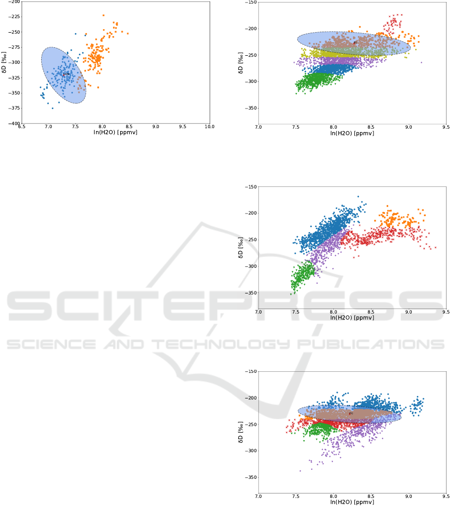
Figure 6: Grid cell at latitude 50 degrees South to 30 de-
grees South and longitude 140 degrees East to 160 degrees
East at 2014-02-15. The ellipse visualizes the cluster prop-
erties of the moving cluster.
tioned at the beginning of this section, the definition
of a moving cluster has been generalized to one spa-
tial neighbour and one time lag, in our case one day.
But each step in our model can be adjusted to the
premise of the analysis; for example by imposing dif-
ferent spatial structures and temporal slices (Step 1),
varying the number of mixture components (Step 2),
applying and adjusting different cluster algorithms for
clustering the mixture components properties (Step
3) and analysing the clusters of cluster properties ac-
cording to the definition of the motion (Step 4), in-
cluding more complex search patterns such as tra-
jectories across multiple spatial regions with varying
timestamps, which will be explored in future work.
5.2.2 Tracking Emerging Clusters
By comparing clusters of the same group in the same
spatial region over time we can also identify emerging
and disappearing clusters. For example if we search
for occurrences over three consecutive days, where a
cluster has been identified on the first and third day,
but not on the second day. One example of an emerg-
ing cluster is given in Figure 7, 8 and 9.
Detecting emerging, disappearing and reappear-
ing clusters with varying cluster properties in cli-
matology data can be a strong indicator for emerg-
ing, disappearing and reappearing climatology events.
In the presented case the emerging and disappearing
cluster in the {H
2
O, δD} feature space can be asso-
ciated with atmospheric water transport due to mix-
ing of air masses with distinctive isotopologue finger-
prints.
Figure 7: Grid cell at latitude 30 degrees South to 10 de-
grees South and longitude 160 degrees West to 140 degrees
West at 2014-02-15. Cluster is present.
Figure 8: Grid cell at latitude 30 degrees South to 10 de-
grees South and longitude 160 degrees West to 140 degrees
West at 2014-02-16. Cluster is absent.
Figure 9: Grid cell at latitude 30 degrees South to 10 de-
grees South and longitude 160 degrees West to 140 degrees
West at 2014-02-17. Cluster is present again.
5.2.3 Tracking Changing Clusters
The proposed approach allows additionally to com-
pare statistics of cluster properties within the same
group and across cluster groups. By looking at
the mean, standard deviation, minimum, maximum
Application of Mixtures of Gaussians for Tracking Clusters in Spatio-temporal Data
51

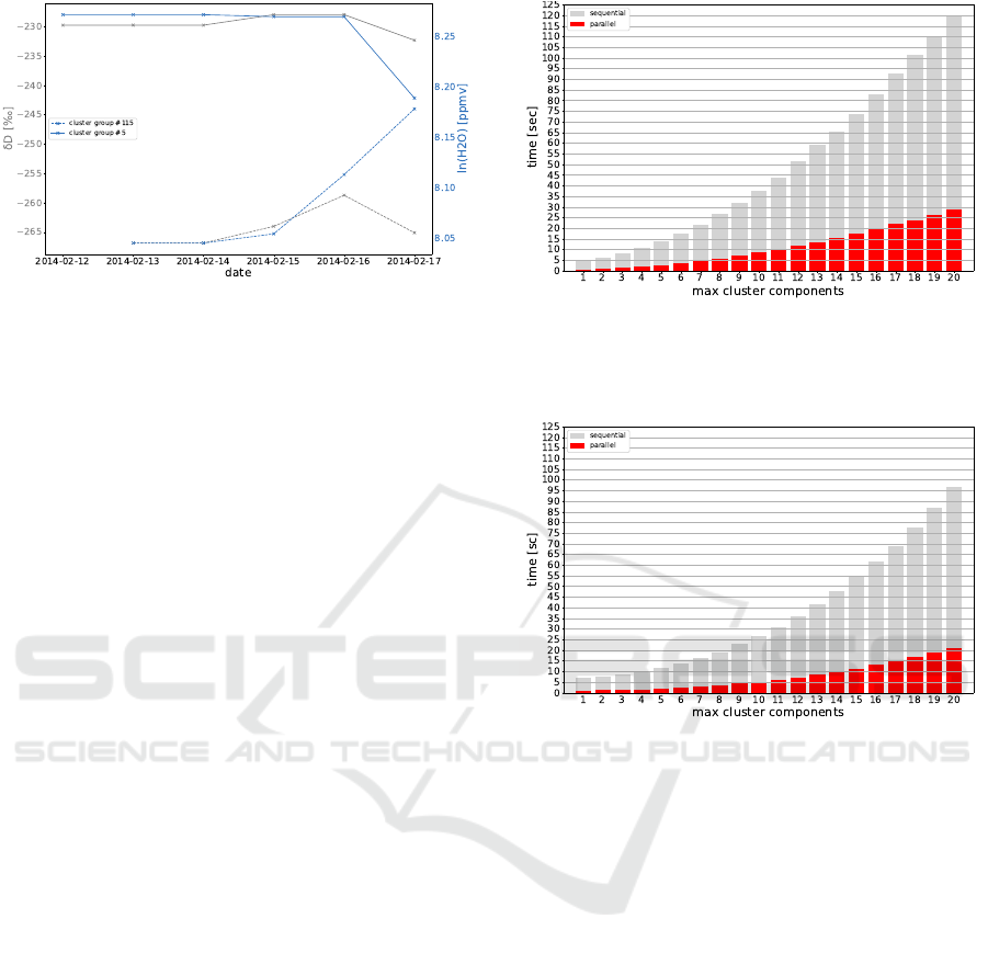
Figure 10: Temporal changes of ln(H2O) as an example
variable over five consecutive days within different cluster
groups. Continuing trends across cluster groups give indi-
cations of cluster evolution.
and percentiles of the identified clusters within the
same group and across groups, these statistical mea-
sures can provide valuable insight into the variability
of cluster properties and possible inference between
clusters and associated climatology events.
We can look for example at the temporal changes
of cluster properties of any cluster group to identify
trends in the cluster features. If the trends are con-
tinuously decreasing or increasing, we can analyse if
the next closest cluster group can be considered an
evolution of the original cluster group. Figure 10 il-
lustrates this on the basis of the temporal changes of
ln(H2O) as an example variable over five consecu-
tive days within two different cluster groups. While
the variable δD for both example cluster groups (#115
and #5) does not show an apparent trend, the ln(H2O)
variable for both cluster groups seem to converge to
the same level. This can give rise to further in-depth
analysis of both cluster groups to explore possible in-
teractions between them.
5.3 Runtime Measurements
As stated in Section 3 each mixture model for any
ROI can be computed in parallel, which decreases the
overall runtime significantly. To demonstrate the scal-
ability of the model, we run tests on both the real data
and synthetic data sequentially with increasing num-
ber of maximum mixture components and in paral-
lel. Figure 11 and Figure 12 illustrates the increasing
amount of computational time necessary with the in-
creasing number of maximum mixture components,
starting from one up to 20 components.
The measurements have been taken on a ordinary
workspace computer with eight Intel
c
Xeon
c
CPU
E3-1246 v3 cores and 32 GB main memory. For the
sequential execution of fitting the GMM models to
one spatial region after another one CPU core was
Figure 11: Sequential and parallel runtime with increasing
maximum number of GMM cluster components for the cli-
matology dataset. The runtime plotted is the time measured
for the best run out of seven runs.
Figure 12: Sequential and parallel runtime with increasing
maximum number of GMM cluster components for the cli-
matology dataset. The runtime plotted is the time measured
for the best run out of seven runs.
busy for up to around two minutes for the real dataset
and around 95 seconds for the synthetic dataset. Run-
ning the GMM fitting for eight spatial regions in par-
allel by distributing the work as separate processes on
all eight cores reduced the runtime significantly by at
least a factor of four, providing the same overall re-
sults.
Figure 13 shows the decreasing runtime with in-
creasing number of CPUs. The number of Gaussian
mixture components has been set to 20 for all runs.
We can see, that the maximum gain has been achieved
with four cores, while adding more cores decreases
the runtime more slowly towards the minimum time
required to analyse one single spatial cell.
By looking at the runtime measurements, we can
conclude that our approach scales well with the num-
ber of spatial regions computed in parallel. While
an increasing number of maximum mixture compo-
nents requires an almost quadratic increasing amount
of time, the overall computational time can be signif-
KDIR 2019 - 11th International Conference on Knowledge Discovery and Information Retrieval
52

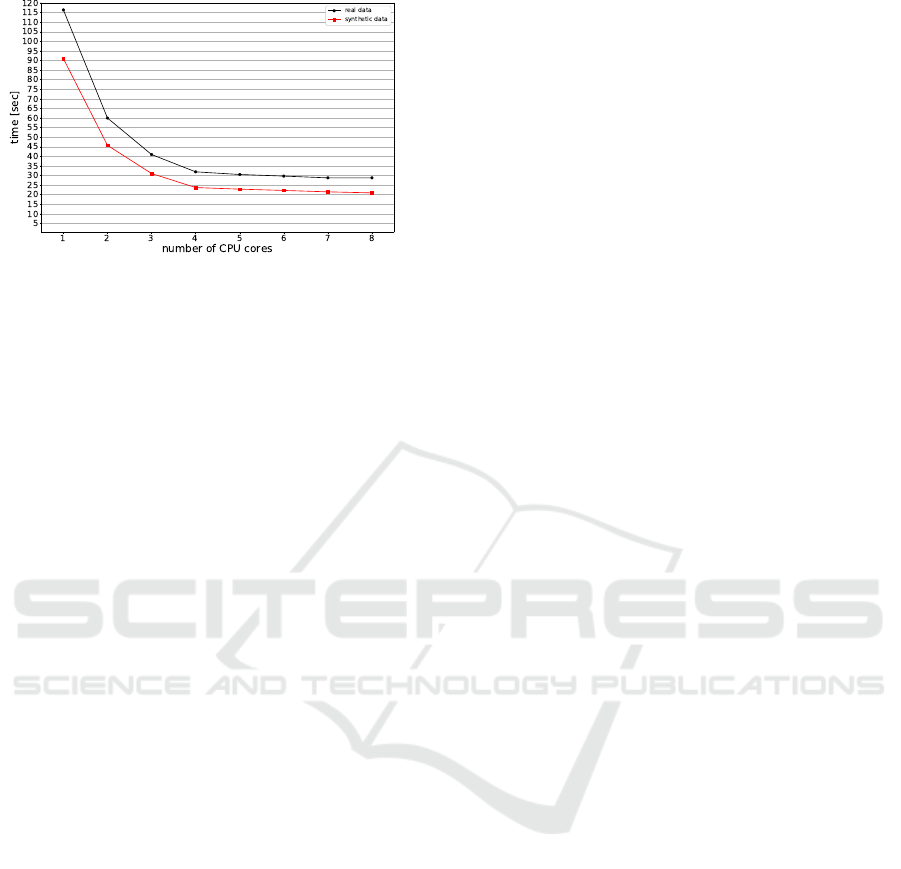
Figure 13: Runtime with different numbers of CPU cores
for the real and synthetic dataset. The maximum number of
GMM components is fixed to 20. The runtime plotted is the
time measured for the best run out of seven runs.
icantly decreased by running the GMM fits for each
spatial region in parallel.
These results highlight the scalability of our ap-
proach which becomes more and more important with
the increasing amount of data that needs to be anal-
ysed. In fact, even if splitting the data in spatial
regions of interest (ROI) might not be applicable,
analysing sub-samples can be done in parallel as well.
By uniform random sampling or biased sampling the
operation of general data mining tasks like clustering
can be significantly speed up (Kollios et al., 2003).
6 DISCUSSION
The initial step of our proposed model, dividing the
data in spatial regions of interest, allows the paral-
lel computation of Gaussian mixture models per area,
which considerably increases the scalability of the ap-
proach. Even if dividing the data into spatial regions
before applying the Gaussian mixture model might
not always be applicable, for example if splitting the
data has a significant effect on the mixture compo-
nents by including or excluding certain observations.
In these cases an analysis of the point generating pro-
cess can help to determine, if the edge-effects can be
statistically evaluated and mitigated (Diggle, 2013).
To further improve the scalability of our model,
each Gaussian mixture model could theoretically be
run in parallel. Instead of sequentially evaluating the
BIC score, the model with the best BIC score could
be selected from parallel computations. Future work
will take this into account to analysis datasets span-
ning over several years as compared to several days
presented in this paper.
The results of the experimental evaluation in Sec-
tion 3 show that our approach is able to successfully
detect changes in cluster properties over space and
time. The examples illustrated in Section 5.2 iden-
tify clusters moving between neighbouring spatial re-
gions with similar cluster properties according to the
applied DBSCAN algorithm on all extracted cluster
properties. Although the proposed approach is not
restricted to any method for comparing the Gaus-
sian mixture components properties, DBSCAN shows
good results and has the advantages that the number
of clusters has not to be specified as a model param-
eter and the E ps and MinPts parameters can be fine-
tuned according to the cluster properties.
While identifying spatio-temporal changes suc-
cessfully, one drawback of our proposed approach is
that modelling the data with mixtures of Gaussians
with the number of components dependent on the
model BIC score is not necessarily describing the un-
derlying process that generated the data accurately.
Therefore the interpretation of the results additionally
relies on domain knowledge associating cluster and
cluster changes to processes.
The utilization of more specific models that can
also capture the underlying data generating processes
more accurately is part of ongoing research.
7 CONCLUSION
In this article we present a scalable approach for
tracking clusters in spatio-temporal data. The pre-
sented method models the observed data in each spa-
tial region with a mixture of Gaussians and compares
extracted cluster properties over time. By dividing the
initial dataset into spatial regions or applying sam-
pling techniques such as random uniform sampling
or biased sampling, each subset can be processed in-
dependently and in parallel, which significantly im-
proves the overall runtime of the proposed model.
As verified on synthetic data with known data gen-
erating processes and applied to real world climatol-
ogy data, the proposed model can reliable detect clus-
ter changes over space and time, indicating moving
clusters, appearing and disappearing events as well as
evolution of clusters over time.
In the future, we plan to apply different Bayesian
models in exchange for the Gaussian mixture model
to incorporate more a priori domain specific knowl-
edge to better catch the underlying processes that gen-
erated the data. Also a more in-depth evaluation in
regard to the scalability of the proposed concept is
planned to be discussed in follow-up work, together
with a detailed evaluation of the clustering results and
their application to climate research.
Application of Mixtures of Gaussians for Tracking Clusters in Spatio-temporal Data
53

REFERENCES
Attias, H. (1999). Inferring parameters and structure of la-
tent variable models by variational bayes. In Proceed-
ings of the Fifteenth conference on Uncertainty in ar-
tificial intelligence, pages 21–30. Morgan Kaufmann
Publishers Inc.
Bishop, C. M. (2006). Pattern Recognition and Machine
Learning. Springer New York.
Chen, S. S. and Gopalakrishnan, P. S. (1998). Clustering via
the bayesian information criterion with applications in
speech recognition. In Acoustics, Speech and Signal
Processing, 1998. Proceedings of the 1998 IEEE In-
ternational Conference on, volume 2, pages 645–648.
IEEE.
Dempster, A. P., Laird, N. M., and Rubin, D. B. (1977).
Maximum likelihood from incomplete data via the
EM algorithm. Journal of the royal statistical soci-
ety. Series B (methodological), pages 1–38.
Diggle, P. J. (2013). Statistical analysis of spatial and
spatio-temporal point patterns. CRC Press.
Ester, M., Kriegel, H.-P., Sander, J., and Xu, X. (1996).
A density-based algorithm for discovering clusters in
large spatial databases with noise. pages 226–231.
AAAI Press.
EUMETSAT (2018). Metop design - IASI.
Greenspan, H., Goldberger, J., and Ridel, L. (2001). A con-
tinuous probabilistic framework for image matching.
Comput. Vis. Image Underst., 84(3):384–406.
Jin, H., Leung, K.-S., Wong, M.-L., and Xu, Z.-B. (2005a).
Scalable model-based cluster analysis using clustering
features. Pattern Recognition, 38(5):637–649.
Jin, H., Wong, M.-L., and Leung, K.-S. (2005b). Scal-
able model-based clustering for large databases based
on data summarization. IEEE Transactions on Pat-
tern Analysis and Machine Intelligence, 27(11):1710–
1719.
Kalnis, P., Mamoulis, N., and Bakiras, S. (2005). On
discovering moving clusters in spatio-temporal data.
In International Symposium on Spatial and Temporal
Databases, pages 364–381. Springer.
Kollios, G., Gunopulos, D., Koudas, N., and Berchtold,
S. (2003). Efficient biased sampling for approxi-
mate clustering and outlier detection in large data sets.
IEEE Transactions on Knowledge and Data Engineer-
ing, 15(5):1170–1187.
Kullback, S. (1997). Information theory and statistics.
Courier Corporation.
Li, Y., Han, J., and Yang, J. (2004). Clustering moving
objects. In Proceedings of the tenth ACM SIGKDD
international conference on Knowledge discovery and
data mining, pages 617–622. ACM.
Maciag, P. S. (2017). A survey on data mining methods for
clustering complex spatiotemporal data. In Interna-
tional Conference: Beyond Databases, Architectures
and Structures, pages 115–126. Springer.
Maimon, O. Z. H., editor (2010). Data mining and knowl-
edge discovery handbook. Springer, New York, 2. ed.
edition.
McLachlan, G. and Peel, D. (2004). Finite mixture models.
John Wiley & Sons.
McLachlan, G. J. and Basford, K. E. (1988). Mixture
models: Inference and applications to clustering, vol-
ume 84. Marcel Dekker.
Paci, L. and Finazzi, F. (2018). Dynamic model-based clus-
tering for spatio-temporal data. Statistics and Com-
puting, 28(2):359–374.
Rey, S. J. and Anselin, L. (2007). PySAL: A Python Li-
brary of Spatial Analytical Methods. The Review of
Regional Studies, 37(1):5–27.
Schneider, M., Borger, C., Wiegele, A., Hase, F., Garc
´
ıa,
O. E., Sep
´
ulveda, E., and Werner, M. (2017). Mu-
sica metop/iasi {H
2
O,δD} pair retrieval simulations
for validating tropospheric moisture pathways in at-
mospheric models. Atmospheric Measurement Tech-
niques, 10(2):507–525.
Trevor, H., Robert, T., and JH, F. (2009). The elements of
statistical learning: data mining, inference, and pre-
diction. Springer.
Zhang, T., Ramakrishnan, R., and Livny, M. (1996). Birch:
an efficient data clustering method for very large
databases. In ACM Sigmod Record, volume 25, pages
103–114. ACM.
KDIR 2019 - 11th International Conference on Knowledge Discovery and Information Retrieval
54