
An Improvement in a Local Observer Design for Optimal State Feedback
Control: The Case Study of HIV/AIDS Diffusion
Paolo Di Giamberardino and Daniela Iacoviello
Dept. Computer, Control and Management Engineering Antonio Ruberti, Sapienza University of Rome, via Ariosto 25,
00185 Rome, Italy
Keywords:
Nonlinear Systems, Linear Observer, Optimal Control, LQR, Epidemic Spread.
Abstract:
The paper addresses the problem of an observer design for a nonlinear system for which a preliminary linear
state feedback is designed but the full state is not measurable. Since a linear control assures the fulfilment of
local approximated conditions, usually a linear observer is designed in these cases to estimate the state with
estimation error locally convergent to zero. The case in which the control contains an external reference, like
in regulations problems, is studied, showing that the solution obtained working with the linear approximation
to get local solutions produces non consistent results in terms of local regions of convergence for the system
and for the observer. A solution to this problem is provided, proposing a different choice for the observer
design which allows to obtain all conditions locally satisfied on the same local region in the neighbourhood of
a new equilibrium point. The case study of an epidemic spread control is used to show the effectiveness of the
procedure. The linear control with regulation term is present in this case because the problem is reconducted to
a Linear Quadratic Regulation problem. Simulation results show the differences between the two approaches
and the effectiveness of the proposed one.
1 INTRODUCTION
The problem of the state measure for dynamical sys-
tems is an important aspect in the control theory for
all the applications in which the control laws require
the knowledge of a non fully measurable state. The
history of solutions to this problem begins with the
case of linear dynamics (Luenberger, 1964) and, less
than ten years later, it is enriched with the first results
for nonlinear ones.
Afterwards, several solutions have been presented
in literature for the design of state observers. Clearly,
the most large number of contributions refers to the
case of nonlinear dynamics, for which nonlinear so-
lutions have been proposed. One direction of the re-
search activity is represented by nonlinear solutions
which mainly follows the idea initially proposed in
(Luenberger, 1964) for linear systems: an observer
can be designed starting from a copy of the dynamics
whom corrective terms are added to, aiming at the sta-
bilization of the linear approximation of the observer
and of the full interconnected system. Examples are
(Andrieu and Praly, 2006), (Zeitz, 1987) and (Sun-
darapandian, 2006), where autonomous dynamics are
considered. The importance of the stabilization of the
linear part of the whole dynamics as an initially local
solution is usually put in evidence separating explic-
itly the linear component of the system from the re-
maining nonlinear terms to better highlight the local
behaviours, (Kazantzis and Kravaris, 1997). A fur-
ther example of a solution based on the possibility of
linearising the error dynamics is represented by (Re-
spondek et al., 2004).
The explicit presence of the input in the non-
linear dynamics usually complicates the approaches,
since suitable bounding conditions must be given, or
different solutions (Sundarapandian, 2002) must be
adopted, modelling the input as generated by an ex-
osystem with known structure.
The list of references could be very long, till
nowadays with, for example, (Sassano and Astolfi,
2019), where an approximated linearising feedback
for the system dynamics is introduced.
In the larger part of their use, observers are part
of feedback control schemes providing a state esti-
mate for state feedback laws. Then, the control design
and the observer determinations are two problems that
must be solved at the same time. They can be solved
separately in the linear case, where the Separation
Principle allows to prove that the addition of an ob-
100
Di Giamberardino, P. and Iacoviello, D.
An Improvement in a Local Observer Design for Optimal State Feedback Control: The Case Study of HIV/AIDS Diffusion.
DOI: 10.5220/0007934501000111
In Proceedings of the 16th International Conference on Informatics in Control, Automation and Robotics (ICINCO 2019), pages 100-111
ISBN: 978-989-758-380-3
Copyright
c
2019 by SCITEPRESS – Science and Technology Publications, Lda. All rights reserved

server does not change the dynamical characteristics
of the controlled system. In the nonlinear case, the
Separation Principle can be also invoked once local
liner approximations are considered, bringing back
the problem to a linear one but restricting to local so-
lutions.
The problem addressed in this paper refers to
the cases in which the nominal state feedback, de-
signed for satisfying prefixed requirements, changes
the equilibrium point of the controlled system. In
this case, the concept of local solution is no more
valid since there exist at least two different reference
points: the equilibrium for the initial given dynamics
and the new one, the working point, equilibrium for
the controlled system.
The approach here followed aims at defining a
unique equilibrium point so that local conditions on
both the control and on the observer can be satisfied
in a neighbourhood of such a point.
Only local conditions are considered, strictly de-
pendent on the regions in which they are defined and
satisfied. Extensions to nonlinear observers can be
performed adopting the same procedure known for
many nonlinear approaches which start with the ful-
filment of local specifications.
The proposed procedure is applied to a case study,
represented by the control of an epidemic spread of a
virus, the one responsible of HIV/AIDS infections.
The choice is motivated by the fact that the clas-
sical procedure, based on the linearisation of the non-
linear dynamics and the design of both the controller
and the observer, satisfying local requirements, per-
formed on the basis of the linearised system, has been
proposed in (Di Giamberardino and Iacoviello, 2018)
and can be assumed as a reference behaviour to com-
pare the solutions here proposed.
A further motivation is that, despite the mathemat-
ical models of different epidemic spreads have pe-
culiar characteristics for each different epidemic ad-
dressed, the control strategy usually adopted in liter-
ature makes reference to optimal solutions, like (Jun,
2006; Bakare et al., 2014; Di Giamberardino and Ia-
coviello, 2017) for the SIR (Susceptible-Infectious-
Removed subjects), (Lin et al., 2010; Gupar and
Quanyan, 2013; Iacoviello and Stasio, 2013) for the
influenza, (Supriatna et al., 2016) for the dengue, and
so on.
The reason of such a choice is that in these cases
the control actions, represented for example by pre-
vention, vaccination, medication, quarantine, are all
subject to a possible limitation and the distribution of
the resources among the different controls can be han-
dled by means of suitable cost functions.
To better understand the mathematical model of
the particular case study adopted, some concepts are
shortly reported. The HIV/AIDS virus attacks the
cells of the immune system, damaging them so that
the immune system is inhibited and the individual is
less protected against other infections. Virus trans-
mission is facilitated by contacts with infected body
fluids. The AIDS represents the most advanced stage
of the HIV infection; it can be reached in 10-15 years
from the initial HIV infection. Up to now, the control
actions are the prevention and the medication after a
positive diagnosis.
The mathematical modelling of the HIV/AIDS
diffusion among populations is focused on the dy-
namic of interactions between individuals (Wodarz
and Nowak, 1999; Pinto and Rocha, 2012; Di Gi-
amberardino et al., 2017; Di Giamberardino et al.,
2018).
In classical HIV/AIDS spread models (Naresh
et al., 2009; Wodarz and Nowak, 1999; Chang and
Astolfi, 2009), four main classes are introduced: the
Susceptible subjects (S), that are the healthy people
that may contract the virus, the Infectious one (I) that
are individuals not aware of their condition, the pre-
AIDS patients (P), the AIDS patients (A). The con-
trol actions introduced are mainly focused on the pre-
vention, as for example in (Rutherford et al., 2016),
where the attention is devoted to risky subjects, drug
users and sex workers.
In this paper, the model proposed in (Di Giamber-
ardino et al., 2017; Di Giamberardino et al., 2018)
and used in (Di Giamberardino and Iacoviello, 2018)
is adopted, for comparative purpose. The main dif-
ference between this and the classical models is that
the susceptible individuals, S, are here divided into
two categories, distinguishing those who adopts wise
behaviours from the ones that do not take into ac-
count the dangerousness of the disease. Moreover,
the model follows the suggestions of the World Health
Organization (WHO) for the control input: i. actions
aiming at reducing the possibility of new infections,
through informative campaign, for example; ii. fa-
cilitations of a fast diagnosis for unaware infectious
patients, thus reducing the percentage of subjects re-
sponsible of the virus spread; iii. medication support
to the aware infectious subjects.
Following (Di Giamberardino and Iacoviello,
2018), the control problem is formulated in the frame-
work of optimal control theory, introducing a cost
function which weights the number of unaware infec-
tious individuals I(t) and the controls introducing a
quadratic cost index. This particular form suggested
to find a solution in the context of a LQR problem,
passing through the linearisation of the dynamics in a
neighbourhood of one of its equilibrium points. The
An Improvement in a Local Observer Design for Optimal State Feedback Control: The Case Study of HIV/AIDS Diffusion
101

solution is a linear state feedback with a constant ref-
erence contribution arising from the regulation prob-
lem.
Unfortunately, for its implementation, the control
scheme needs a state observer, since only the num-
ber of the patients with HIV (P) and AIDS (A) are
available. As already discussed, the observer design
can be performed working on the model linearisation
already adopted for the LQR problem solution, as in
(Di Giamberardino and Iacoviello, 2018).
This approach and the improvement introduced to
overcome some consequent consistency problems are
discussed in the paper. More in details, in Section
2 the inconsistencies of the straightforward approach
which works on the same linearised dynamics are put
in evidence, while the improvements for overcoming
such a problem are presented and discussed in Sec-
tion 3. The procedure is then applied to the case study
in Section 4, comparing it with the simpler classical
one. Some results of numerical simulations are re-
ported in Section 5 to validate the proposed solution.
Some concluding remarks in Section 6 end the paper.
2 PROBLEM DEFINITION
Given the nonlinear dynamics
˙x = f (x) + g(x)u (1)
y = h(x) (2)
with x ∈ ℜ
n
, u ∈ ℜ
m
, y ∈ ℜ
p
, and the equilibrium
point x
e
( f (x
e
) = 0, g(x
e
) 6= 0, h(x
e
) = 0), the prob-
lem here studied refers to the case in which the design
of an observer is required for the implementation of a
state feedback control. As discussed in the Introduc-
tion, the majority of the approaches for the determi-
nation of an observer for a nonlinear system aims at
obtaining local asymptotic convergence, in a neigh-
bourhood of one equilibrium point, with the addition
of further conditions on the strictly nonlinear part of
the dynamics, and on the input, when necessary, to ex-
tend the region of convergence or to make the result
global.
So, if one restricts the attention to linear feedback
control law, satisfactory once only local conditions
on the control are required, then also for the observer
the design can be restricted to satisfy local conditions
only, so simplifying the computation and, sometimes,
its implementation.
Under these hypothesis, the problem can be ap-
proached computing firstly the linear approximation
of (1)–(2), getting
˙
˜x = A ˜x + Bu
˜y = C ˜x (3)
where, as usual, A =
∂ f
∂x
x=x
e
, B = g(x
e
), C =
∂h
∂x
x=x
e
,
˜x = x − x
e
and ˜y = y − Cx
e
. Based on (3), the linear
feedback control and the linear observer can be easily
computed working in the linear context.
In the present work, the case in which the linear
feedback control computed assumes the form
u = K ˜x + r (4)
is considered. The linear term K ˜x satisfies the local
stability of the controlled system in a neighbourhood
of the equilibrium point. The additional presence of
a forcing constant term r in (4) is considered, which
usually appears when dealing with a regulation prob-
lem, where the external input plays the role of a ref-
erence value. In Section 4 a real case is introduced to
show an example of synthesis in which the regulation
term naturally appears.
In this case of whole linear approximation and lo-
cal solutions, the closed loop dynamics under state
measurement would become
˙
˜x = (A + BK)˜x + Br (5)
The linear observer may assume the classical Luen-
berger form (Luenberger, 1964)
˙
˜z = (A − GC)˜z +Bu +G˜y (6)
The dynamics of the error e = ˜z − ˜x locally in a neigh-
bourhood of x
e
is described by
˙e = (A − GC)˜z + Bu + G ˜y −(A + BK)˜x − Br =
= (A − GC)e (7)
asymptotically convergent to zero once σ(A − GC) ∈
C
−
. Then, the asymptotic condition lim
t→∞
k˜z − ˜xk = 0
holds and it can be rewritten as
lim
t→∞
k˜z − ˜xk = lim
t→∞
k˜z + x
e
− x k = 0 (8)
showing that if ˜z is the estimate of ˜x, then z = ˜z + x
e
is
the estimate of the original state x.
Remaining in the approximated context, the whole
system obtained using the state reconstructed by the
observer in the control law (4) is described by
˙
˜x = A ˜x + BK ˜z + Br
˙
˜z = (A − GC)˜z + BK ˜z + Br + GC ˜x (9)
and, replacing the observer dynamics with the one of
the estimation error e = ˜z − ˜x, the full dynamics is
given by
˙
˜x = (A + BK)˜x + BKe + Br
˙e = (A − GC)e (10)
that is the proof of the Separation Principle.
ICINCO 2019 - 16th International Conference on Informatics in Control, Automation and Robotics
102

This procedure has been used in (Di Giamber-
ardino and Iacoviello, 2018) for the optimal control
of an epidemic spread. The example is recalled in
next Section 4 and it is used to show the new result
discussed later in the paper.
A weakness of the procedure described above can
be put in evidence once the solution is applied to the
original nonlinear model.
In order to analyse the effects of each contribution
in the whole controlled system, the use of the nominal
state feedback (4) is firstly introduced. The controlled
dynamics can be written as
˙x = f (x) + g(x) (K(x − x
e
) + r) = F
c
(x,r) (11)
Computing the equilibrium points, denoted as x
c
e
to put in evidence its origin from the controlled dy-
namics, one has
f (x
c
e
) + g(x
c
e
)(K(x
c
e
− x
e
) + r) = F
c
(x
c
e
,r) = 0 (12)
It is easy to verify that if r = 0, x
c
e
= x
e
. Otherwise,
the new equilibrium point x
c
e
is different from x
e
.
This change implies that, at steady state, the sys-
tem is in the equilibrium point x
c
e
.
The introduction of an observer to estimate the
state for a feedback implementation must preserve
this asymptotic behaviour, as it happens in the linear
case, and the equilibrium point must remain x
c
e
.
The fulfilment of this condition can be verified
analysing the whole system obtained introducing the
estimated state given by the observer for the state
feedback (13) applied to system (1).
On the basis of the relationships between the local
state ˜x and its estimate ˜z, as well as between the orig-
inal state x and its estimate z, the control law (4) can
be expressed, in the original coordinates, as
u = Kz − Kx
e
+ r (13)
and the observer dynamics (6) can assume the form
˙z = (A − GC)(z − x
e
) + Bu + Gy − GCx
e
=
= (A − GC)z − Ax
e
+ Bu + Gy (14)
The full interconnected dynamics is then de-
scribed by
˙x = f (x) + g(x)Kz − g(x)Kx
e
+ g(x)r
˙z = (A − GC + BK)z − (A + BK)x
e
+ GCx + Br
(15)
In order to check the effectiveness of the con-
trolled system (15), as a first step the error dynamics
like (7) can be computed to verify its convergence to
zero.
˙e = (A − GC + BK − g(x)K)e
+(A + BK − g(x)K)x − f (x)
−(A + BK − g(x)K)x
e
+ (B − g(x))r
(16)
Approximating (16) in a neighbourhood of x = x
e
, one
gets
˙e = (A − GC)e (17)
the same as in (10) as expected. That is, while the
system converges to x
e
, the estimation error goes to
zero.
The problem is that, for the full dynamics (15), x
e
is not an equilibrium point, as it is easy to verify just
substituting x = x
e
in
f (x) + g(x)Kz − g(x)Kx
e
+ g(x)r = 0
(A − GC + BK)z − (A + BK)x
e
+ GCx + Br = 0
(18)
as well as z = x
e
since the estimation error goes to
zero. The condition
Br = 0 (19)
is obtained, clearly impossible. On the other hand, not
even x = x
c
e
, and then z = x
c
e
, are equilibrium condi-
tions for the two subsystems because, by substitution
in (18), the expressions
−g(x
c
e
)Kx
e
= 0
(A + BK)(x
c
e
− x
e
) + Br = 0
(20)
are obtained, again impossible.
It is possible to conclude that this approach cannot
work properly because i. the insertion of the observer
dynamics interferes with the characteristics of the
controlled system, changing the equilibrium point; ii.
the observer does not work as expected, since the
manifold in which the local convergence is assures
does not coincide with a neighbourhood of the new
equilibrium point.
The goal of the present paper is to introduce an
improvement in the procedure recalled above, remain-
ing in the locally linearised approximated context but
avoiding the undesired effects i. and ii. described
above.
3 THE PROPOSED DESIGN
PROCEDURE
The idea followed for the solution here proposed is
based on the possibility of designing a state observer
in such a way that the equilibrium point of the con-
trolled system is the same both when the state is sup-
posed to be measured and when its estimate provided
by the observer is used.
Starting from the system (1)–(2), suppose it has
been defined a linear state feedback control with a
An Improvement in a Local Observer Design for Optimal State Feedback Control: The Case Study of HIV/AIDS Diffusion
103

regulation term of the form (4), expressed in the orig-
inal coordinates,
u = Kx + r (21)
The controlled dynamics is described by
˙x = f (x) + g(x)Kx + g(x)r = F(x, r) (22)
with output (2). Using the same notation previously
adopted, be x
c
e
the equilibrium point for the controlled
system (22), F(x
c
e
,r) = 0.
The design technique is again based on a linear
observer and on local convergence of the estimation
error, but preserving the convergence of the system to
x
c
e
.
To this aim, the linear approximation of (22) in a
neighbourhood of x
c
e
is computed as
˙
¯x = A
c
¯x (23)
where
¯
A =
∂F(x,r)
∂x
x=x
c
e
and ¯x = x − x
c
e
. Now, a linear
observer is designed on the basis of the closed loop
system, i.e. an observer for the state of (22). The
structure is the same as in (6), so that it has the form
˙
¯z = A
c
¯z + G( ¯y −C¯z) = (A
c
− GC)¯z + G ¯y (24)
where ¯y = y − Cx
c
e
is defined as in the previous case
for a different equilibrium point. Conditions under
which the estimation error converges asymptotically
to zero for the so defined problem are trivial, being
σ(A
c
− GC) ∈ C
−
.
The so obtained observer is used in the full closed
loop system to provide a state estimation for the state
feedback (21). Clearly, since ¯z is the estimation of
¯x, that is lim
t→∞
k ¯x − ¯zk = 0, z = ¯z + x
c
e
is the estimation
of x; in fact lim
t→∞
k ¯x − ¯zk = lim
t→∞
k(x − x
c
e
) − (z − x
c
e
)k =
lim
t→∞
kx − zk = 0
In order to study the effect of such a control
scheme, the full closed loop dynamics has to be writ-
ten. One has
˙x = f (x) + g(x)Kz + g(x)r
= F(x,r) + g(x)K(z − x)
˙z = (A
c
− GC)z − A
c
x
c
e
+ GCx (25)
If the dynamics of the error e = z − x is computed,
the expression
˙e = (A
c
− GC)(e + x) − A
c
x
c
e
+ GCx − F(x,r)
−g(x)Ke =
= (A
c
− GC − g(x)K)e + A
c
(x − x
c
e
) − F(x, r)
(26)
is obtained. Its approximation in a neighbourhood of
x = x
c
e
can be computed, setting
F(x,r) = A
c
(x − x
c
e
) (27)
and
B
c
= g(x
c
e
) (28)
so yielding
˙e = (A
c
− GC − B
c
K)e (29)
which converges, if the pair (A
c
− B
c
K,C) is de-
tectable, finding G such that σ(A
c
−B
c
K − GC) ∈ C
−
.
At the same time, once the equilibrium points of
(25) are computed, it is easy to verify, by straight-
forward substitution, that x = x
c
e
and z = x
c
e
are one
solution. In fact
F(x
c
e
,r) + g(x
c
e
)K(x
c
e
− x
c
e
) = 0
(A
c
− GC)x
c
e
− (A
c
− GC)x
c
e
= 0
The fulfilment of the Separation Principle can be ver-
ified, rewriting (25) in the new coordinates (x,e):
˙x = F(x,r) + g(x)Ke
˙e = (A
c
− GC − g(x)K)e + A
c
(x − x
c
e
) − F(x, r)
(30)
which, in a neighbourhood of x = x
c
e
can be approxi-
mated as
˙x = A
c
x + B
c
Ke − A
c
x
c
e
˙e = (A
c
− GC − B
c
K)e
(31)
whose dynamical matrix is
A
TOT
=
A
c
B
c
K
0 A
c
− GC − B
c
K
(32)
proving that the Separation Principle still holds.
A comparison between the two approaches, the
first with the equilibrium point change and an error
on the state estimation, and the second, for which the
equilibrium is left unchanged and the Separation Prin-
ciple holds, is reported in next Section 4. In particu-
lar, the first approach is recalled referring to (Di Gi-
amberardino and Iacoviello, 2018) and it is used to
compare the results obtained with the here proposed
design procedure.
4 THE CASE STUDY
4.1 A Short Recall of the Mathematical
Model
In this paper, the model of the HIV/AIDS diffusion
presented in (Di Giamberardino et al., 2017; Di Gi-
amberardino et al., 2018) is adopted and is here briefly
recalled. Main characteristics of this epidemic are the
ICINCO 2019 - 16th International Conference on Informatics in Control, Automation and Robotics
104

possibility of spread limitation by means of a healthy
behaviour of individuals, while vaccination is still not
available; moreover, there can be a quite long period
during which infected persons are infective but un-
conscious of their status, since the symptoms appear
later.
The first point motivates the introduction of a con-
trol based on suitable informative and educational
campaign, to reduce unhealthy relationships, instead
of a more classical vaccination action, and of a con-
trol aiming to discover infected individuals as soon as
possible, through a blood test campaign.
The state variables introduced in the model de-
note the healthy people S
1
, not aware of dangerous
behaviours and then can be infected, and S
2
, the ones
that, suitably informed, give great attention to the pro-
tection, and the three levels of infectious subjects: I,
the infective but unaware of their status, P, the HIV
positive patients, A, the AIDS diagnosed ones.
As previously discussed, the control actions are
the information campaign, u
1
and the test campaign
to discover the infection as soon as possible, u
2
. A
third action, u
3
, the therapy which aims at reducing
the transition from HIV to AIDS, is also considered,
since mortality among A is higher that in P.
Then, the mathematical model is
˙
S
1
= Z − dS
1
− β
S
1
I
N
c
+ γS
2
− S
1
u
1
˙
S
2
= −(γ + d)S
2
+ S
1
u
1
˙
I = β
S
1
I
N
c
− (d + δ)I − ψ
I
N
c
u
2
˙
P = εδI − (α + d)P + φψ
I
N
c
u
2
+ Pu
3
˙
A = (1 − ε)δI + αP − (µ + d)A +
+(1 − φ)ψ
I
N
c
u
2
− Pu
3
(33)
where N
c
= S
1
+ S
2
+ I. In (33), d denotes the rate of
natural death; Z denotes the flux of new subjects in the
class S
1
; β is related to the dangerous interactions be-
tween S
1
and I categories; γ is the rate of wise subjects
that could change, incidentally, their status, increas-
ing S
1
(t); ψ is related to the control action aiming at
helping the individuals in class I to discover their in-
fectious condition, and therefore to flow to the P or
the A class; φ is the percentage of test positive sub-
jects with HIV ((1 − φ) the percentage with AIDS); δ
is the rate of transition from I to P (percentage ε) or A
(percentage (1 − ε)) without any external action; α is
the rate of the natural transition from P to A; µ is the
rate of death in class A caused by the infection.
Dynamics (33) can also be expressed in the com-
pact form
˙
X = f (X) + g(X)U = F(X,U) (34)
once X = (S
1
S
2
I P A)
T
, U = (u
1
u
2
u
3
)
T
and
f (X) =
Z − dS
1
−
βS
1
I
N
c
+ γS
2
−(γ + d)S
2
βS
1
I
N
c
− (d + δ)I
εδI − (α + d)P
(1 − ε)δI + αP − (µ + d)A
(35)
g(X) =
g
1
g
2
g
3
=
−S
1
0 0
S
1
0 0
0 −ψ
I
N
c
0
0 φψ
I
N
c
P
0 (1 − φ)ψ
I
N
c
−P
(36)
are defined.
For the definition of possible output functions, it
must be observed that the subject with a positive diag-
nosis, P and A, can be easily measured, since reported
by medical operators. On the other hand, individuals
I cannot be known at all: they can be discovered only
after blood test or symptoms rise, but in these case
they are counted as P or A. Consequently, also S
1
and
S
2
can be known. The entire population is another
measurable quantity.
Then, it seems reasonable to assume the measure
of the total number of diagnosed individuals, P(t) +
A(t), as the possible meaningful output, so giving
y(t) = CX(t), C =
0 0 0 1 1
(37)
4.2 The Control Problem Formulation
In this Section the control problem is shortly dis-
cussed showing one of the cases in which the con-
trol law is a linear state feedback with an additional
constant reference term. An optimal control problem
for the HIV/AIDS dynamics (33) has been formulated
in (Di Giamberardino and Iacoviello, 2018) under the
following assumptions: i. the most dangerousness as-
pect in the epidemic spread is represented by the in-
dividuals I, so that their minimization was the main
goal; ii. once a diagnosis is given, there is no dif-
ference between P and A with respect to the decre-
ment of I, so the therapy u
3
does not influence I at all
and it will be not considered, setting it to zero (any
value would have the same effects on I). Then, the
two–dimensional control vector
ˆ
U = (u
1
u
2
)
T
is intro-
duced, neglecting, consequently, the vector field g
3
(·)
in (36), introducing also the matrix ˆg(X) =
g
1
g
2
.
An Improvement in a Local Observer Design for Optimal State Feedback Control: The Case Study of HIV/AIDS Diffusion
105

Under these positions, the cost function
J(X,
ˆ
U) =
1
2
Z
∞
t
0
qI
2
+ r
1
u
2
1
+ r
2
u
2
2
dt =
=
1
2
Z
∞
t
0
X
T
QX +
ˆ
U
T
R
ˆ
U
dt (38)
is defined, with Q the five dimensional square ma-
trix with all zero entries except Q(3,3) = q, and
R =
r
1
0
0 r
2
, r
1
,r
2
> 0. In other words, the goal
of the proposed control action is the minimization of
the number of infectious subjects I making use of as
less resources as possible.
The quadratic structure of (38) and the preference
for a state feedback implementability of the control
law drove the solution of such problem in (Di Gi-
amberardino and Iacoviello, 2018) to a LQR form de-
signed on the linearised approximation of (33) in the
neighbourhood of one equilibrium point.
A study of the existence of equilibrium points
and of their stability properties has been performed
in (Di Giamberardino et al., 2017; Di Giamberardino
et al., 2018), yielding to the two possible solutions
X
e
1
=
1/d
0
0
0
0
Z X
e
2
=
1/H
0
H−d
H(d+δ)
εδ(H−d)
H(α+d)(d+δ)
δ(H−d)[(1−ε)d+α]
H(α+d)(d+δ)(µ+d)
Z
(39)
where H = β − δ. The non negativeness of the el-
ements in the vector state X
e
2
implies the conditions
H > 0 and H ≥ d; therefore the equilibrium point X
e
2
is a feasible one if and only if H ≥ d, being X
e
1
= X
e
2
if H = d. A bifurcation analysis is reported in (Di Gi-
amberardino et al., 2018).
Making use of the same values for the model
parameters as in (Di Giamberardino and Iacoviello,
2018), condition H > d holds, so that both the equilib-
rium points exist. Computing the two linearised dy-
namics in the neighbourhood of the two equilibrium
points one gets
˙
˜
X = A
i
˜
X +
ˆ
B
i
ˆ
U
˜y = C
˜
X (40)
with A
i
=
∂F
∂X
,
ˆ
B
i
=
∂F
∂
ˆ
U
= ˆg, all evaluated at X = X
e
i
and
ˆ
U = 0, ˜y = C
˜
X = y −CX
e
i
and
˜
X = X − X
e
i
(41)
i = 1, 2 depending on the choice.
Despite the procedure can be adopted making ref-
erence to both the equilibrium points, easy computa-
tions show that the linear dynamics which approxi-
mates the nonlinear one in the neighbourhood of X
e
1
is neither detectable nor controllable. So, in view of
a control synthesis in the local linear domain, the lin-
earisation in a neighbourhood of X
e
2
is chosen. Then,
the linear dynamics is (40) with i = 2.
4.3 The Optimal Control Problem
Solution
The use of the new coordinates
˜
X, consequence of
(41), implies a change of variables also in the cost
function (38), where
˜
X must appear instead of X. The
new expression is
J(X,
ˆ
U) = J(
˜
X + X
e
2
,
ˆ
U) =
˜
J(
˜
X,
ˆ
U) =
=
1
2
R
∞
t
0
˜
X
T
− ¯r
Q
˜
X − ¯r
+
ˆ
U
T
R
ˆ
U
dt
=
1
2
R
∞
t
0
q
˜
I(t) +
H−d
H(d+δ)
2
+ r
1
u
2
1
(t)+ r
2
u
2
2
(t)
dt
(42)
where ¯r = (∗ ∗ ¯r
˜
I
∗ ∗)
T
denotes the LQR tracking
term, with ¯r
˜
I
= −
H−d
H(d+δ)
.
For a dynamics (40), the optimal control problem
with cost function (42) corresponds to a classical Lin-
ear Quadratic Regulator (LQR) problem with a con-
stant tracking term.
The result, computed and discussed in (Di Gi-
amberardino and Iacoviello, 2018), is a state feedback
control law with a reference term. Once the Algebraic
Riccati Equation
0 = K
R
ˆ
B
2
R
−1
ˆ
B
T
2
K
R
− K
R
A
2
− A
T
2
K
R
− Q (43)
is solved w.r.t. K
R
, the state feedback optimal control
law is given by ((Anderson and Moore, 1989))
ˆ
U = −R
−1
ˆ
B
T
2
K
R
˜
X + R
−1
ˆ
B
T
2
g
¯r
=
= K
˜
X + r
(44)
where g
¯r
=
K
R
ˆ
B
2
R
−1
B
T
2
− A
T
2
−1
Q ¯r and Q ¯r =
(0 0 q
¯r
˜
I
0 0)
T
, K = −R
−1
ˆ
B
T
2
K
R
is the gain matrix as in
(4) while r = R
−1
ˆ
B
T
2
g
¯r
is the constant tracking term r.
Stability for the linear controlled system is proven
in (Di Giamberardino and Iacoviello, 2018). In the
same paper, the problem of the unavailability of a
measure of all the state variables has been solved
computing a linear state observer under the hypoth-
esis that, once only local solutions are available, due
to the request of a state feedback control, then also
for the observer a linear approach can be sufficient,
whose approximation is well compensated by its sim-
plicity of design and implementation.
Then, once verified the detectability property on
(A
2
,C) in (40) (i = 2), the state estimation ˜z(t)
of the state
˜
X verifying the asymptotic condition
lim
t→+∞
k
˜
X(t) − ˜z(t)k = 0 can be obtained as the state
evolution of the Luenberger like linear observer
˙
˜z(t) = (A
2
− GC) ˜z(t) +
ˆ
B
2
ˆ
U(t) + G ˜y(t) (45)
ICINCO 2019 - 16th International Conference on Informatics in Control, Automation and Robotics
106

with matrix G chosen in order to have all the eigen-
values of the dynamic matrix (A
2
−GC) with negative
real part.
The whole control system is a dynamical output
feedback control with state observer and feedback
from the state estimation.
4.4 Improved Observer Design
Following what illustrated in Section 3, consider the
control law of the form (44) computed solving the
LQR control problem on the basis of the linear ap-
proximation of the dynamics in a neighbourhood of
X
e
2
is obtained. Under the action of this state feed-
back, the controlled system assumes the form
˙
X = f (X) + ˆg(X)(K
˜
X + r) = F(X,r) (46)
with its linear approximation asymptotically sta-
ble. Its equilibrium point can be denoted by X
c
e
:
F(X
c
e
,r) = 0 and the linear approximation of (46) in
the neighbourhood of X
c
e
can be computed; it is given
by
˙
¯
X = A
c
¯
X (47)
where A
c
=
∂F(X ,r)
∂X
X=X
c
e
and
¯
X = X − X
c
e
.
A local linear observer for the linear approximat-
ing dynamics can be designed in the usual form
˙
¯z = (A
c
− GC)¯z + G ¯y (48)
when dealing directly with the linearised dynamics,
or
˙z = (A
c
− GC)z + Gy − A
c
X
c
e
(49)
expressed in the original state variables and their esti-
mations.
According to the general discussion in Section 3,
once the observer has been designed, the control law
(44) should be implemented using the state estimate
¯z instead of the real but not measurable state
¯
X (or
z instead of X). Then the control law (44) has to be
rewritten as
u = K
˜
X + r = K(X − X
e
2
) + r =
= K(
¯
X + X
c
e
− X
e
2
) + r =
= K
¯
X + r + K(X
c
e
− X
e
2
) (50)
so that the dynamics (46) under the employment of
the observer (48), assumes the expression
˙
X = f (X) + ˆg(X)(K ¯z + r) + ˆg(X)K(X
c
e
− X
e
2
) (51)
to be considered along with the observer dynamics
(48). Some manipulations allow to write the dynam-
ics (51) as
˙
X = f (X) + ˆg(X)(K ¯z + r) + ˆg(X)K(X
c
e
− X
e
2
) =
= F(X,r) + ˆg(X)K(¯z −
˜
X + X
c
e
− X
e
2
) =
= F(X,r) + ˆg(X)K(z − X) (52)
where z−X can be replaced by ¯z −
¯
X or ˜z−
˜
X accord-
ing to the convenience. It is easy to verify by substitu-
tion that the whole dynamics (48)–(52) has the equi-
librium point X = X
c
e
, z = X
c
e
(
¯
X = ¯z = 0). This means
that asymptotically the state of the observer and one
of the original system are equal. The fact that the
asymptotic error is equal to zero can be proved also
computing the error dynamics
˙e = (A
c
− GC)¯z + GC ¯x − F(X,r) − ˆg(X)K(z − x)
(53)
and evaluating it in a neighbourhood of X = X
c
e
, yield-
ing
˙e = (A
c
− GC)¯z + GC ¯x − A
c
¯x −
ˆ
B
c
K(¯z − ¯x) =
= = (A
c
− GC +
ˆ
B
c
K)e (54)
Then, with σ(A
c
− GC +
ˆ
B
c
K) ∈ C
−
the error goes
asymptotically to zero.
It is confirmed what stated in the previous Section:
the observer (48) works properly, without producing
undesired changes in the system dynamics and con-
verging asymptotically to the system state, once G is
designed to have σ(A
c
− GC −
ˆ
B
c
K) ∈ C
−
, provided
that (A
c
−
ˆ
B
c
K,C) is a detectable pair.
5 NUMERICAL RESULTS AND
DISCUSSION
In this Section, a numerical analysis is performed to
show the effectiveness of the proposed solution and to
compare it with the previous more classical one.
The values for the parameters in the dynamics (33)
adopted for the numerical computations have been
taken, for comparative purposes, from (Di Giamber-
ardino and Iacoviello, 2018; Naresh et al., 2009;
Di Giamberardino et al., 2017); they have been firstly
used in (Massad, 1989) on the basis of epidemio-
logical research conducted at the San Francisco City
Clinic:
d = 0.02, β = 1.5, δ = 0.4, ε = 0.6
φ = 0.95, γ = 0.2 ψ = 10
5
, α = 0.5
µ = 1, Z = 1000 (55)
Then, H = β − δ = 1.1 > 0 so that the equilibrium
point X
e
2
exists and it is locally asymptotically stable.
Numerically, X
e
2
= (0.91 0 2.34 1.08 0.9)
T
· 10
3
.
The linear approximation in the neighbourhood of
this equilibrium point is described by the following
An Improvement in a Local Observer Design for Optimal State Feedback Control: The Case Study of HIV/AIDS Diffusion
107

numerical matrices:
A
2
=
−0.80 0.20 −0.12 0 0
0 −0.22 0 0 0
0.78 0 0.30 0 0
0 0 0.24 −0.52 0
0 0 0.16 0.5 −1.02
(56)
ˆ
B
2
=
−0.91 0
0.91 0
0 −72
0 68.40
0 3.60
10
3
(57)
while C is already expressed in a linear form with re-
spect to X in (37).
As far as the controller is concerned, the control
law is computed as the solution of the LQR problem
with offset (tracking) term defined in Subsection 4.3
once the controllability property has been checked.
It is easy to verify that for A
2
,
ˆ
B
2
in (56) and (57) it
holds.
Performing the computations, the LQR reference
term ¯r
˜
I
to be used in (44) assumes the value ¯r
˜
I
=
−2.34 · 10
3
.
The weights q = 10
−4
, r
1
= 1, r
2
= 1000 are cho-
sen in the cost function; motivations can be found in
(Di Giamberardino and Iacoviello, 2018).
The solution K
R
of the Algebraic Riccati Equation
(43) gives
K
R
=
0.07 −0.01 0.14 0 0
−0.01 0.02 −0.05 0 0
0.14 −0.05 4.33 0 0
0 0 0 0 0
0 0 0 0 0
10
−6
(58)
and then g
¯r
=
0.05 0 −1.03 0 0
T
· 10
−2
.
The optimal control (44) so obtained, which
should drive the state variable
˜
I of the linearised sys-
tem to the reference value ¯r
˜
I
, is of the form (44) with
K = 10
−4
−0.71 0.25 −1.78 0 0
−0.10 0.04 −3.12 0 0
(59)
and
r =
0.41
0.74
(60)
Taking into account the state transformation (41),
the linear state feedback control law is computed.
When dealing with the observer design, for com-
parative purpose firstly the previously available solu-
tion is recalled in Subsection 5.1 and then the results
of the implementation of the one proposed in this pa-
per are reported and discussed.
5.1 The Classical Solution
For this solution, the property of detectability for the
pair (56) and (37) must be verified. For the present
numerical values it can be verified that it holds.
Then, the design procedures for the state observer
can be performed.
Since the solution here adopted is based on the
use of a linear state observer, the design procedure
requires the computation of matrix G in (45) such that
the matrix (A
2
− GC) is asymptotically stable.
Discussion about the characteristics of the tran-
sient in the observer dynamics are reported in
(Di Giamberardino and Iacoviello, 2018) and they
bring to the choice of the set of eigenvalues Λ =
{
−1.0, −1.1, −1.2, −1.3, −1.4
}
to be assigned to
the matrix (A
2
− GC). The corresponding numerical
value of G is
G =
4.18 15.31 14.87 2.19 1.56
T
(61)
5.2 The Proposed Solution
Following the procedure described in Section 3, the
observer to be designed has the form (24) rewritten as
in (25) and here reported for the present case
˙z = (A
c
− GC)z + GCx − A
c
X
c
e
(62)
where G has to be computed, according to (29), after
having verified the detectability property for the pair
(A
c
− B
c
K,C), in order to have σ(A
c
− B
c
K − GC) ∈
C
−
.
The first step of the procedure is the computation
of the equilibrium point X
c
e
for the controlled system
(46) under the hypothesis of a state feedback. For the
numerical case here addressed, it is
X
c
e
= 10
4
1.0176 3.9822 0 0 0
T
(63)
For the computation of the matrix A
c
− B
c
K, A
c
has to be computed as the Jacobian of the controlled
system evaluated in (63), B
c
= g(X
c
e
), while K is the
output of the LQR optimal control problem previ-
ously solved. Performing all the computations, one
gets
A
c
=
1.09 0.21 1.04 0 0
−1.11 −0.23 −1.34 0 0
0 0 −0.34 0 0
0 0 0.24 −0.52 0
0 0 0.16 0.50 −1.02
(64)
ICINCO 2019 - 16th International Conference on Informatics in Control, Automation and Robotics
108
and, then,
A
c
+ B
c
K =
=
1.04 0.21 0.92 0 0
−1.06 −0.23 −1.22 0 0
−0.76 −0.01 −23.40 0 0
0.72 0.01 22.15 −0.52 0
0.04 0 1.31 0.50 −1.02
(65)
It can be checked that
rank
C
C(A
c
+ B
c
K)
C(A
c
+ B
c
K)
2
C(A
c
+ B
c
K)
3
C(A
c
+ B
c
K)
4
= 5 (66)
and then it is possible to compute G so to verify the
convergence condition. With the same choice as in
the previous case for the eigenvalues of the error dy-
namics one has
G = 10
3
−0.22 1.20 0.03 −0.02 0
T
(67)
The following Section is devoted to the numerical
simulations and the discussion of the results.
5.3 Simulation Results
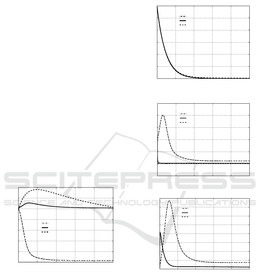
0 10 20 30 40 50
0
1
2
3
4
5
6
7
x 10
4
Time t
S
1
(t)
Linear observer
Proposed method
State feedback
Figure 1: Time history of individuals in S
1
(t).
Three cases have been simulated to compare their
behaviours. One obviously is the application of the
procedure proposed in the paper, denoted in the leg-
end of the Figures 1–5 by Proposed method. The nu-
merical values used are the ones reported in the pre-
vious Subsection 5.2. The effectiveness of the con-
trol scheme can be confirmed by the results depicted
in the Figures with the solid lines. In fact, its action
produces a fast reduction of the infected I, Figure 3,
and, consequently, a decrease of the number of the
diagnosed patients P, Figure 4, and A, Figure 5. At
the same time, the number of healthy individuals S
1
0 10 20 30 40 50
0
0.5
1
1.5
2
2.5
3
x 10
4
Time t
S
2
(t)
Linear observer
Proposed method
State feedback
Figure 2: Time history of individuals in S
2
(t).
0 10 20 30 40 50
−0.5
0
0.5
1
1.5
2
2.5
x 10
4
Time t
I(t)
Linear observer
Proposed method
State feedback
Figure 3: Time history of individuals in I(t).
0 10 20 30 40 50
0
2000
4000
6000
8000
10000
12000
14000
16000
Time t
P(t)
Linear observer
Proposed method
State feedback
Figure 4: Time history of individuals in P(t).
is maintained sufficiently high, Figure 1, while, due
to a reduction of the infection probability, the passage
from S
1
to S
2
is no more necessary for the spread con-
tainment and the individuals in S
2
, reported in Figure
2, naturally tend to zero by natural death.
Two other cases have been considered. One is the
same reported in (Di Giamberardino and Iacoviello,
2018), while the other one is the case in which the
state is supposed fully measurable and then the feed-
back control law can be directly implemented without
the necessity of a state observer.
An Improvement in a Local Observer Design for Optimal State Feedback Control: The Case Study of HIV/AIDS Diffusion
109
0 10 20 30 40 50
0
1000
2000
3000
4000
5000
6000
7000
8000
9000
10000
Time t
A(t)
Linear observer
Proposed method
State feedback
Figure 5: Time history of individuals in A(t).
For each of the five state variables, the results of
the simulation for these two cases are reported: the
dash-dot line, marked with Linear observer, is de-
voted to depict the time histories of the state variables
in the case of application of the procedure addressed
in Subsection 5.1, the one of the previous cited work;
the dashed line, for which the denomination in the
legend is State feedback, depicts the behaviours of the
state variables when the feedback control law is ap-
plied using directly a state measurement. These two
cases are useful to compare the thee procedures, since
in the case of State feedback any negative effect of the
observer is avoided, showing the powerful of the con-
trol strategy only, while making use of the results for
the Linear observer case, it is possible to appreciate
the advantages of centring the linear approximation
of the observer in correspondence to the new equilib-
rium point arising from the control action.
6 CONCLUSIONS
This paper discusses the problem of the implemen-
tation of a state feedback control using an asymp-
totic state observer. The case in which, for the solu-
tion of the control problem, a linear approximation of
the dynamics in a neighbourhood of one equilibrium
point is the natural framework, also a local linear ob-
server is proposed. The contribution of the paper is
in the presentation of the case in which the applica-
tion of the controller changes the equilibrium point
so that, for higher performances, the determination
of the linear approximation for the observer design
can make use of the knowledge of the new final equi-
librium point where the controlled system asymptot-
ically converges. The effectiveness of the proposed
solution is also evidenced from the results of numer-
ical simulations, where it is possible to note that in
this case the behaviours of the controllers with and
without the observer are very similar.
REFERENCES
Anderson, B. D. O. and Moore, J. B. (1989). Optimal con-
trol.
Andrieu, V. and Praly, L. (2006). On the existence of a
Kazantis-Kravaris/Luenberger observer. SIAM Jour-
nal on Control and Optimization, 45(2):432–456.
Bakare, E. A., Nwagwo, A., and Danso-Addo, E. (2014).
Optimal control analyis of an SIR epidemic model
with constant recruitment. International Journal of
Applied Mathematical Research, 3.
Chang, H. and Astolfi, A. (2009). Control of HIV infection
dynamics. IEEE Control Systems Magazine.
Di Giamberardino, P., Compagnucci, L., Giorgi, C. D., and
Iacoviello, D. (2017). A new model of the HIV/AIDS
infection diffusion and analysis of the intervention ef-
fects. 25
th
IEEE Mediterranean Conference on Con-
trol and Automation.
Di Giamberardino, P., Compagnucci, L., Giorgi, C. D., and
Iacoviello, D. (2018). Modeling the effects of pre-
vention and early diagnosis on HIV/AIDS infection
diffusion. IEEE Transactions on Systems, Man and
Cybernetics: Systems.
Di Giamberardino, P. and Iacoviello, D. (2017). Optimal
control of SIR epidemic model with state dependent
switching cost index. Biomedical Signal Processing
and Control, 31.
Di Giamberardino, P. and Iacoviello, D. (2018). LQ con-
trol design for the containment of the HIV/AIDS dif-
fusion. Control Engineering Practice, 77.
Gupar, E. and Quanyan, Z. (2013). Optimal control of in-
fluenza epidemic model with virus mutation. Euro-
pean Control Conference.
Iacoviello, D. and Stasio, N. (2013). Optimal control for
SIRC epidemic outbreak. Computer Methods and
Programs in Biomedicine.
Jun, J. H. (2006). Optimal synthesize control for an SIR
epidemic model. 24
th
IEEE Chinese Control and De-
cision Conference.
Kazantzis, N. and Kravaris, C. (1997). Nonlinear observer
design using Lyapunov’s auxiliary theorem. Proc.
36
th
Conference on Decision & Control.
Lin, F., Muthuraman, K., and Lawley, M. (2010). Optimal
control theory approach to non-pharmaceutical inter-
ventions. BNC Infectious Diseases, 10(32):1–13.
Luenberger, D. G. (1964). Observing the state of a linear
system. IEEE Trans. on Military Electronics, MIL-
8(2):74–80.
Massad, E. (1989). A homogeneously mixing population
model for the AIDS epidemic. Math. Comput. Mod-
elling.
Naresh, R., Tripathi, A., and Sharma, D. (2009). Modeling
and analysis of the spread of AIDS epidemic with im-
migration of HIV infectives. Mathematical and Com-
puter Modelling, 49.
Pinto, C. and Rocha, D. (2012). A new mathematical model
for co-infection of malaria and HIV. 4th IEEE Inter-
national Conference on Nolinear Science and Com-
plexity.
ICINCO 2019 - 16th International Conference on Informatics in Control, Automation and Robotics
110

Respondek, W., Pogromsky, A., and Nijmeijer, H. (2004).
Time scaling for observer design with linearizable er-
ror dynamics. Automatica, 40.
Rutherford, A. R., Ramadanovic, B., Michelow, W., Mar-
shall, B. D. L., Small, W., Deering, K., and Vasarhe-
lyi, K. (2016). Control of an HIV epidemic among in-
jection drug users: simulations modeling on complex
networks. 2016 Winter Simulations Conference.
Sassano, M. and Astolfi, A. (2019). A local separation prin-
ciple via dynamic approximate feedback and observer
linearization for a class of nonlinear systems. IEEE
Trans. Aut. Control, 64(1):111–126.
Sundarapandian, V. (2002). Local observer design for non-
linear systems. Mathematical and Computer Mod-
elling, 35.
Sundarapandian, V. (2006). Reduced order observer design
for nonlinear systems. Applied Mathematics Letters,
19.
Supriatna, A. K., Anggriani, N., Mlanie, and Husniah, H.
(2016). The optimal strategy of Wolbachia-infected
mosquitoes release program. 2016 Int. Conf. on In-
strumentation, Control and Automation (ICA).
Wodarz, D. and Nowak, M. (1999). Specific therapy
regimes could lead to long-term immunological con-
trol of HIV. Proc. Nat. Acad. Sci., 96(25):14464–
14469.
Zeitz, M. (1987). The extended Luenberger observer for
nonlinear systems. Syst. and Contr. Lett., 9.
An Improvement in a Local Observer Design for Optimal State Feedback Control: The Case Study of HIV/AIDS Diffusion
111
