A Method for Static and Dynamic Interval Detection within the IMU

Calibration Procedure

Andrejs Zujevs, Valters Vecins and Aleksandrs Korsunovs

Riga Technical University, Kalku iela 1, Riga, Latvia

Keywords:

IMU, MEMS, Calibration, Static Detector.

Abstract:

An Inertial Measuring Unit (IMU) is used for measuring linear accelerations and angular velocities in 3D/2D

space. IMU devices are usually designed as micro-electro-mechanical systems (MEMS), which are produced

in small form factor and are widely used in robotics, mobile phones and drones. Depending on the quality

of the device, they can be divided into low-cost and high-cost IMUs. The main difference between them is

the accuracy of measurements and IMUs mechanical alignment on the printed circuit board. The high-cost

IMUs are well calibrated and have a relatively small error and noise level for different kinds of parameters.

In contrast, the low-cost IMUs have a larger error component, where body frame axes are non-orthogonal

for both the accelerometer and gyroscope due to weak factory calibration, high noise and high sensitivity de-

pendence from the temperature, misalignment of body frame due to packaging and assembly processes. This

paper provides a new method for the IMU static and dynamic interval detection within the IMU calibration

procedure, which is designed by other authors for the case of IMU calibration without any external equipment.

This procedure uses a sequence of alternating static and dynamic intervals for accelerometer calibration and

then gyroscope calibration. The accuracy of the IMU calibration procedure depends strongly on how precisely

static and dynamic intervals have been detected. Otherwise, the calibration results are unsuitable. The new

method for static and dynamic interval detection provides more robust and less noisy results, requires a sig-

niﬁcantly smaller number of operations and is easy to implement. The paper provides comparative results for

both methods and refers to the source code for the new method.

1 INTRODUCTION

An Inertial Measurement Unit (IMU) is a sensor used

for measuring linear accelerations and angular veloc-

ities in 3D/2D space. With the help of these measure-

ments, it is possible to track changes in sensor rotation

and translation. One of the main applications of the

IMU is providing information about an objects body

frame orientation in global coordinates with no addi-

tional information about the world. Since the current

state evaluation using only an IMU depends on the ac-

curacy of the previous state evaluation, it is thus prone

to error accumulation. Usually, for additional local-

isation information, IMU data are fused with other

sensors onboard a mobile robot, a drone, or another

mobile platform (Le Gentil et al., 2018). The most

recent applications of IMU have been in the ﬁeld of

visual odometry and visual-inertial SLAM (Qin et al.,

2018; Mur-Artal and Tardos, 2016; Vidal et al., 2017).

As part of the multi-sensor system, an IMU provides

high-frequency measurements, necessary for a robot’s

or drone’s systems to compensate translation or ro-

tation movement, while slower sensors evaluate the

global position. By integrating measured values of an

accelerometer, gyroscope and often a magnetometer,

over time it becomes possible to estimate the move-

ment trajectory (Qin et al., 2018).

IMUs that are used in robotics and mobile

phones are usually based on MEMS (micro-electro-

mechanical systems) technology because of their

small form factor. Most of them are a combination of

several triaxial units: an accelerometer, a gyroscope

and often a magnetometer. The MEMS may be di-

vided in low-cost (up to 5$) and high-cost (starting

from 100$) devices. The main difference between

them is the accuracy of the measurements provided

by the units and the accuracy of the IMUs mechani-

cal alignment on a PCB. The high-cost IMUs are well

calibrated and have a relatively small error component

for the different types of IMU parameters. Also, they

have low error values for misalignment. In contrast,

low-cost IMUs have a larger error component.

Body frame axes are non-orthogonal for both the

accelerometer and the gyroscope) due to weak factory

746

Zujevs, A., Vecins, V. and Korsunovs, A.

A Method for Static and Dynamic Interval Detection within the IMU Calibration Procedure.

DOI: 10.5220/0007929007460751

In Proceedings of the 16th International Conference on Informatics in Control, Automation and Robotics (ICINCO 2019), pages 746-751

ISBN: 978-989-758-380-3

calibration, high noise, sensitivity dependence from

the temperature and misalignment of the body frame

due to packaging and assembly processes. Axis mis-

alignment in a triaxial device (Figure 1) is a major

source of measurement error, which is caused due to

weak factory calibration or/and IMU soldering accu-

racy and alignment on a PCB (Looney, 2015).

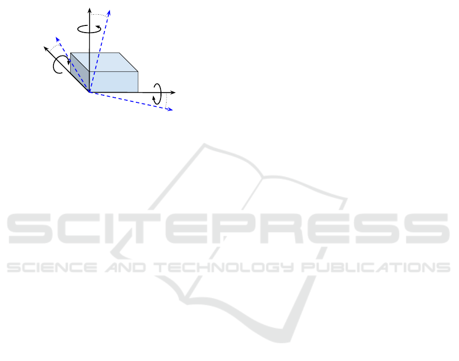
IMU device

z’

x’

y’

Ѱy

Ѱz

Ѱx

Figure 1: Misalignment of IMU device gyroscope’s axes

(dotted blue lines) in right-hand coordinate system. The

ﬁgure adopted from (Looney, 2015), where misaligned axes

are x

, y

, z

and global frame axes are x, y, z and angle Ψ is

the misalignment angle for each axis relative to the global

frame axis. Circular bullets around each global frame axis

show both gyroscope rotation direction and speed for an

axis.

In order to improve IMU performance, it is nec-

essary to perform a calibration procedure in addition

to the factory calibration. Some of the sensors from

the high-price segment come with calibration matri-

ces calculated individually for each sensor in the fac-

tory. Cheaper sensors have less precise calibration,

which should be compensated to achieve the desired

performance. In addition to the IMU parameter cali-

bration, it is necessary to determine the relative posi-

tion of the sensor and the body frame.

The best calibration results can be achieved

by utilising dedicated calibration tools. Chambers

with temperature control and very precise multi-axis

turntables allow to calibrate and compensate most

of IMU parameters such as non-orthogonality (Deng

et al., 2017). However, since the operation of such

equipment is expensive, it is not accessible for every

researcher. Also, it is unfounded for cheaper IMUs

because of the difference in the precision grade of the

equipment and the sensor that needs to be calibrated.

Systems that use multiple sensors can be cal-

ibrated by performing an inter-sensor calibration.

When multiple sensors perform measurements of the

same quantity using different phenomena, those mea-

surements can be cross-validated in order to achieve

better precision and use the more suited sensor as a

reference to calibrate the parameters of the other sen-

sor (Lv, J., Ravankar, A.A., Kobayashi, Y., Emaru,

2016). Similarly, by performing body frame position

evaluation with multiple sensors, it is possible to com-

pensate for inter-sensor spatial and temporal offsets

(Furgale et al., 2013).

IMU self-calibration is the simplest method of

calibration in terms of resource utilisation - in most

cases, the only things needed are a ﬂat surface and

an operator. Most of the work in this type of calibra-

tion relies on speciﬁc manoeuvres performed on the

sensor to collect a set of calibration data (Shin and

El-Sheimy, 2002; Ren et al., 2015).

This paper focuses on the low-cost IMU MEMS

calibration method without the use of external equip-

ment, as presented in (Tedaldi et al., 2014). In that

work proposed IMU calibration method solves the

body-frame non-orthogonality cause of errors, also

known as sensor misalignment. This paper provides

an improvement of the static detector described as a

part of the IMU calibration procedure or framework

(Tedaldi et al., 2014). All the experiments and evalua-

tions of the new method were conducted with a device

equipped with mouse-based ADNS-9500 microchip

(optical ﬂow sensor) (Briod et al., 2012; Beyeler and

Floreano, 2009) and LSM6DSL (STMicroelectronics,

2017) IMU device onboard.

2 THE IMU CALIBRATION

PROCEDURE

The IMU calibration procedure proposed in (Tedaldi

et al., 2014) is intended for IMU MEMS calibra-

tion without external equipment. The procedure uses

raw accelerometer and gyroscope data as input data,

which are prepared in a speciﬁc way. An IMU device

is placed in N different static attitudes, where each

lasts for 1-2 seconds. The procedure starts with the

initial static position lasting T seconds, which for a

particular IMU device may vary between 15 - 30 sec-

onds. Then, a sequence of alternating dynamic and

static positions of the IMU device has to be done.

The initial static interval called the initialization pe-

riod is used to ﬁnd an appropriate threshold value of

the accelerometer’s Allan Variance (Barnes and Al-

lan, 1990) magnitude. This threshold value is used

for static intervals detection in the raw accelerome-

ter data. The overall calibration procedure is shown

in Figure 2. The static detector processing the raw

accelerometer data detects a sequence of static inter-

vals (when IMU lies in a static position, without any

movement). The data from the static intervals are then

used as input data in the step of the accelerometer cal-

ibration. The accelerometer rotation, scaling, and bias

matrices are estimated and used in the next step for the

gyroscope calibration. The data within the dynamic

A Method for Static and Dynamic Interval Detection within the IMU Calibration Procedure

747

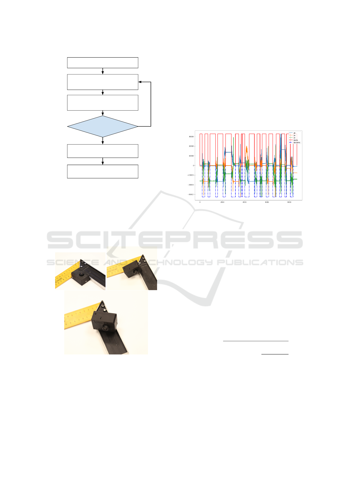
Leave the IMU static for T sec.

Rotate the IMU and then lay it in

a different attitude

Wait for at least M seconds

Have you

rotated the IMU

N times?

Yes

Calibrate Accelerometer

and then Gyroscope

Apply the static interval detector

Figure 2: The overall IMU calibration procedure. Figure

adopted from (Tedaldi et al., 2014).

intervals and data from the calibrated accelerometer

are used as the input data in the gyroscope calibra-

tion. As a result, rotation and scaling matrices are es-

timated (Tedaldi et al., 2014). Figure 3 shows an ex-

ample of raw data gathering when a device equipped

with IMU is sequentially placed in different static at-

titudes for a period of 1-2 seconds.

Figure 3: A device equipped with LSM IMU which was

placed in different static attitude positions.

3 STATIC DETECTOR

The task of the static detector is to determine from

IMU’s raw data such intervals of data when a device

is in a static state (without any movement), and re-

ferred to as a static interval further in this paper. Ac-

cordingly to the calibration procedure, such intervals

of data which are located between neighbour static in-

tervals belong to the IMU movement from one static

position to another and are named as dynamic inter-

vals. Figure 4 shows an example of the detected static

and dynamic intervals, where the accelerometer sig-

nal (within ax, ay and az axes) in a static interval ﬂuc-

tuates around the same value level, and, in contrast, in

a dynamic interval, the signal changes signiﬁcantly.

The accuracy of the calibration depends strongly on

Figure 4: Static intervals determined by the static detector

and the dynamic intervals between them.

the correctness of the determined static and dynamic

intervals. This statement is based on the fact that

(Tedaldi et al., 2014) the accelerometer is calibrated

by using the averages for each axis from static inter-

vals, and the gyroscope is calibrated by using the cal-

ibrated accelerometer data and the gyroscope’s data

integrated within the dynamic intervals. This paper

provides an improvement of the variance based static

detector introduced in (Pretto and Grisetti, 2014).

3.1 The Original Version

The static detector introduced in (Pretto and Grisetti,

2014) is variance based and uses an operator of vari-

ance in magnitude estimation for each accelerometer

sample (a

, a

) at time t:

ς(t) =

[var

)]

+ [var

)]

[var

)]

(1)

where var

) is a variance operator which com-

putes variance of signal a

within a time window

centered at t, t

- length of the time window. The

static and dynamic intervals are classiﬁed based on

the threshold value, simply checking if it is lower or

greater than ς(t) squared. The threshold is an integer

multiplier of the ς

init

squared. The multiplier is esti-

mated within the initialization period T

init

. The length

of the period is determined by estimating the Allan

ICINCO 2019 - 16th International Conference on Informatics in Control, Automation and Robotics

748

variance for each gyroscope axis, where σ

is deﬁned

as:

∑

k=1

(x(

t, k) − x(

t, k − 1))

(2)

where x(

t, k) is k − th interval average which spans

seconds, and K is the number of intervals that the total

considered time is segmented in. The time interval

in which the Allan variances of the three gyroscope

axes converge to a small value may be an appropriate

initialization period T

init

(Tedaldi et al., 2014).

3.2 A New Version

The new version of the static detector

is expressed

in the pseudocode (Algorithm 1). The detector uses

three input parameters t

- a time window for which

magnitude is estimated by 1 eq.; t

- the minimal

length of a static interval in seconds; t

dyn

- the min-

imal length of a dynamic interval in seconds, and

raw accelerometer data with the timestamps of the

records. Estimated magnitude values estimated by 1

eq. are in a relatively large value range. Therefore, it

is better to use a logarithmic function, which reduces

relative differences between values and makes inter-

val detection more robust. In this work, the logarithm

to the base 10 is used. When the magnitude of ac-

celerometer data variance has been evaluated (Figure

5), the value of the magnitude threshold will be es-

timated as magnitude average for values greater than

log(1.0) (small bias). This threshold is used to split

raw data into static and dynamic intervals (Figure 6).

Because of the fact that raw accelerometer data are

usually formed by values in a range of positive and

negative numbers, it’s important to note that we need

to add some bias and make all values positive before

performing the logarithmic magnitude estimation.

3.3 Comparative Analysis

We compared the previous version of the static detec-

tor proposed by (Tedaldi et al., 2014) and our version.

Unfortunately, within this work scope, it is difﬁcult to

provide some quantitative metrics on how well both

detectors performed. To solve this issue, we should

use a manually marked dataset or apply the IMU cal-

ibration procedure on the same dataset using deter-

mined intervals from both detectors. On the other

hand, we may do some comparison based on Fig-

ures and computation time. All experiments were per-

formed on the dataset from our device and with total

of 16343 samples on the host computer equipped with

Intel Core i7 CPU 965 @ 3.20GHz 8 and with 16GB

https://github.com/IKSAResearchLab/IMU Calibration.git

Figure 5: Estimated magnitude by Eq.1 without using loga-

rithm function.

Figure 6: Estimated logarithmic magnitude and the deter-

mined threshold value (the blue horizontal line) used for

splitting data in static and dynamic intervals.

of RAM with the original detector’s MATLAB2018b

program was performed in 64.22 seconds, where the

used value of t

was 9 samples. However, our de-

tector on the same host and a program implemented

in C processes the same dataset in 0.01 seconds. In

our detector, we used t

= 0.05 seconds or a 9-sample

long time period, t

= 1.0 seconds and t

dyn

= 0.4 sec-

onds. The original detector generated too much noise

if t

value was too small as the one mentioned above

(Figure 7), but generated good results if t

was set

to 120 samples long time window, no noise was ob-

served (Figure 8). The new detector is more conﬁg-

urable and it is possible to set the minimal value of

the static and dynamic interval, which reduces noise

A Method for Static and Dynamic Interval Detection within the IMU Calibration Procedure

749

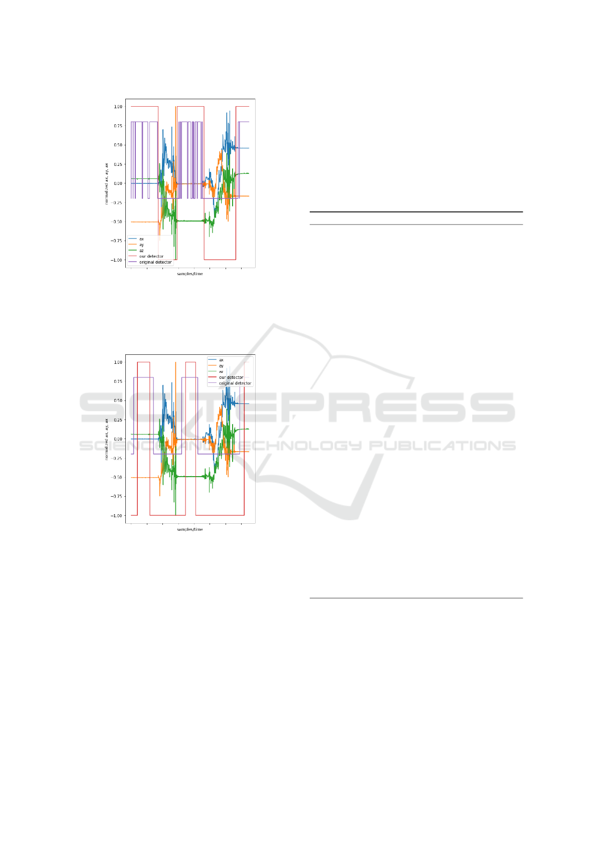
Figure 7: The results of interval detection with both de-

tectors. The sub-window of the overall dataset is shown,

where t

= 0.05 seconds or is 9 samples long. The origi-

nal detector produced noise within the static intervals. The

accelerometer values have been normalized for better rep-

resentation.

Figure 8: The results of intervals detection with both de-

tectors. The sub-window of the overall dataset is shown,

where t

= 0.5 seconds or is 120 samples long. The orig-

inal detector provided good results. The new detector gen-

erated more narrowed intervals than the original one. The

accelerometr’s values were normalized for better represen-

tation.

in detected intervals and, therefore, will improve the

calibration accuracy and increase the quality of the

validation process. Results of the new detector are de-

pended to selected values of t

. If the value is small

as the one used above, then the borders of the static

intervals are more close to the dynamic signals of the

accelerometer. In the case of the high values, on the

contrary, the borders of the static intervals are far from

the dynamic signals of the accelerometer as shown in

Figure 8. After many experiments with both detec-

tors, it has been concluded that the new detector pro-

vides smoother results (is less noisy) than the origi-

nal one. The new detector provides the quality metric

for the detected static intervals. The metric is imple-

mented as a variance operator, which is applied to the

logarithmic magnitude values of a static interval. The

lower this metric value is, the more useful is the static

interval.

Algorithm 1: The new version of static detector.

Require: ACC

(n,3)

dyn

∈ R

1: function GET-MAGNITUDE(ACC,t

)

2:  Returns logarithmic magnitude of ACC

3: M ← hi;m

avg

← 0

4: for all µ ∈ ACC do

5: M

← log

(ς(µ) + 1.0)  see eq. 1

6: end for

7: m

avg

← avg(M) for all M

> b

8: return (M, m

avg

)

9: end function

10: function GET-INTERVALS(M ∈ R

, m

avg

dyn

)

11:  The function detects stat. and dyn. interv.

12: j, k ← 0;

13: S, D ← hi  Stat. and dyn. interv. sequences

14: for all M

∈ M, (0 6 i < m) do

15: if M

≤ m

avg

and len(S

curr

) ≤ t

then

16: Stat

← (start

idx

, stop

idx

)

17: j = j +1

18: end if

19: if M

> m

avg

and len(Dyn

curr

) ≤ t

dyn

then

20: Dyn

← (start

idx

, stop

idx

)

21: k = k + 1

22: end if

23: end for

24: return (S, D)

25: end function

26: (M, m

avg

) ← GET-MAGNITUDE(ACC,t

)

27: (S, D) ← GET-INTERVALS(M, m

avg

dyn

)

28: narrow(S, D, count)  Narrow all static intervals

in S

29: var(S)  Estimate variance of magnitude for all

static intervals (quality metric)

4 CONCLUSIONS

The accuracy of the IMU calibration procedure de-

pends strongly on how precisely static and dynamic

intervals have been determined. The original detector

performs sufﬁciently well if the time window value

interval used in the variance magnitude estimation is

not too small. At the same time, the original detec-

ICINCO 2019 - 16th International Conference on Informatics in Control, Automation and Robotics

750

tor is more computationally expensive, especially if it

is necessary to ﬁnd an appropriate value of the time

window parameter.

The new detector was implemented in C and is

much quicker and easily implementable than the orig-

inal one. It also provides more options for parame-

ter settings. Finally, it provides a quality metric for

the determined static intervals. This metric is useful

in the accelerometer calibration step and in the gy-

roscope calibration step when the triads of static and

dynamic intervals have been selected.

In further research activities, we should make a

numerical analysis of the static detector within the

IMU calibration procedure and compare obtained cal-

ibration accuracy for the proposed and other static de-

tectors.

ACKNOWLEDGEMENTS

This work has been supported by the European Re-

gional Development Fund within the Activity 1.1.1.2

Post-doctoral Research Aid of the Speciﬁc Aid Ob-

jective 1.1.1 To increase the research and inno-

vative capacity of scientiﬁc institutions of Latvia

and the ability to attract external ﬁnancing, invest-

ing in human resources and infrastructure of the

Operational Programme Growth and Employment

(No.1.1.1.2/VIAA/2/18/334).

REFERENCES

Barnes, J. A. and Allan, D. W. (1990). Variances based on

data with dead time between the measurement. NIST

Tech. Note, 1318:296–335.

Beyeler, A. and Floreano, D. (2009). optiPilot : control of

take-off and landing using optic ﬂow. Eur. Micro Air

Veh. Conf. Compet. 2009 (EMAV 2009).

Briod, A., Zufferey, J. C., and Floreano, D. (2012). Au-

tomatically calibrating the viewing direction of optic-

ﬂow sensors. Proc. - IEEE Int. Conf. Robot. Autom.,

pages 3956–3961.

Deng, Z., Sun, M., Wang, B., and Fu, M. (2017). Anal-

ysis and Calibration of the Nonorthogonal Angle in

Dual-Axis Rotational INS. IEEE Trans. Ind. Elec-

tron., 64(6):4762–4771.

Furgale, P., Rehder, J., and Siegwart, R. (2013). Uniﬁed

temporal and spatial calibration for multi-sensor sys-

tems. In 2013 IEEE/RSJ International Conference on

Intelligent Robots and Systems, pages 1280–1286.

Le Gentil, C., Vidal-Calleja, T., and Huang, S. (2018). 3D

Lidar-IMU Calibration Based on Upsampled Prein-

tegrated Measurements for Motion Distortion Cor-

rection. 2018 IEEE International Conference on

Robotics and Automation (ICRA), pages 2149–2155.

Looney, M. (2015). The Basics of MEMS IMU/Gyroscope

Alignment. Analog Dialogue, 49(June):1–6.

Lv, J., Ravankar, A.A., Kobayashi, Y., Emaru, T. (2016).

A method of low-cost IMU calibration and alignment.

SII 2016 - 2016 IEEE/SICE International Symposium

on System Integration, pages pp. 373—-378.

Mur-Artal, R. and Tardos, J. (2016). Visual-inertial monoc-

ular slam with map reuse. IEEE Robotics and Automa-

tion Letters, PP.

Pretto, A. and Grisetti, G. (2014). Calibration and perfor-

mance evaluation of low-cost IMUs. 18th Internation-

alWorkshop on ADC Modelling and Testing.

Qin, T., Li, P., and Shen, S. (2018). VINS-Mono: A Ro-

bust and Versatile Monocular Visual-Inertial State Es-

timator. IEEE Transactions on Robotics, 34(4):1004–

1020.

Ren, C., Liu, Q., and Fu, T. (2015). A Novel Self-

Calibration Method for MIMU. IEEE Sensors Jour-

nal, 15(10):5416–5422.

Shin, E. and El-Sheimy, N. (2002). A new calibration

method for strapdown inertial navigation systems. Z.

Vermess, 127:1–10.

STMicroelectronics (2017). Lsm6dsl datasheet.

Tedaldi, D., Pretto, A., and Menegatti, E. (2014). A ro-

bust and easy to implement method forIMU calibra-

tion without external equipments. Proceedings - IEEE

International Conference on Robotics and Automa-

tion, pages 3042–3049.

Vidal, A. R., Rebecq, H., Horstschaefer, T., and Scara-

muzza, D. (2017). Ultimate SLAM? Combining

Events, Images, and IMU for Robust Visual SLAM

in HDR and High Speed Scenarios. IEEE Robotics

and Automation Letters, 3(2):994–1001.

A Method for Static and Dynamic Interval Detection within the IMU Calibration Procedure

751