Electromyography Signal Analysis to Obtain Knee Joint Angular

Position

Edinson Porras, Lina Peñuela and Alexandra Velasco

Universidad Militar Nueva Granada, Mechatronics Engineering Department, Bogota, Colombia

Keywords:

Electromyography, Knee Rehabilitation, Polynomial Adjustment, Locally Weighted Projection Regression.

Abstract:

Knee injuries are due to several causes and affect a large part of the population. In all of the cases, rehabilitation

is required to recover the joint mobility and strength. In this context, the use of technology, especially the

development of assistive devices may offer advantages to the patients, e.g. allow to perform correctly the

exercises, adapt to the users’ needs and help to comply with the prescribed physical therapy. These devices

may have speciﬁc requirements focused on not harming the patient. This is why control strategies are needed,

and therefore feedback sensing is highly important. In this paper we present an algorithm to determine the

knee joint angular position from surface Electromyography (EMG) measurements, using a curve ﬁt from a

polynomial adjustment method and a Locally Weighted Projection Regression (LWPR) method. We validate

our approach, comparing the data obtained from the curve ﬁtting with the measurements obtained with position

sensors. In this way, results show that indeed we can explain the joint angular position with the EMG data

taken in knee ﬂexion-extension motion, applying a polynomial adjustment approach and the LWPR method.

1 INTRODUCTION

The amount of people suffering knee impairments

caused by accidents, cord injury, arthritis, and aging

is increasing (Koller-Hodac et al., 2010). To recover

partially or completely the normal functions, or to

avoid the joint degeneration, a rehabilitation process

is required in all cases. Part of the treatment includes

physiotherapy, which implies different procedures to

reduce pain and swelling, and to recover mobility and

strength (Huo et al., 2016), (Umivale, 2011). Tra-

ditionally, the subjects must attend limited therapy

sessions that most of the times are not enough to

recover the joints normal function (Jensen and Lor-

ish, 1994). Other times the subjects do not comply

with the prescribed treatment reducing its effective-

ness (Khan and Scott, 2009). Additionally, the treat-

ment evaluation is usually done in a visual or verbal

way, therefore it can be subjective (Umivale, 2011).

In some cases, as part of the treatment the physi-

cian prescribes the use of elements as orthoses, elastic

bands, and so on, to improve the subjects’ condi-

tion. However, the traditional orthoses are rigid struc-

tures which limit the user’s natural motion, and may

cause discomfort. This is why recently, there has

been an increasing interest in the development and

use of assistive robotic devices for physical rehabili-

tation (see e.g. (Fang et al., 2018) or (Koller-Hodac

et al., 2011)), which are oriented to improve the tradi-

tional rehabilitation methods, allowing the treatment

completion, as well as the adaptation to the users’ re-

habilitation process and requirements.

Several assistive devices are already available in

literature. For example, (Ren et al., 2017) address a

wearable ankle robotic device in passive and active

training in acute stroke. As part of the design, authors

report the need of controllers. This device senses and

tracks the patient’s motion (or intent of motion) of

the ankle without harm. It is worth to mention that

important considerations must be made for design-

ing systems oriented to stroke patients; however, this

topic is out of the scope of our paper.

Other assistive devices in literature do not have a

feedback control system, but use measurements (e.g.

electromyography (EMG)) to control the system in

open loop. This is the case of the upper limb exo-

skeleton in (Mghames et al., 2017), which is im-

plemented with a Variable Stiffness Actuator (VSA).

Authors obtain an analogy of the open loop control

parameters with those of the human muscle system,

tuning in that way the mechanical system paramet-

ers. The feed-forward control inputs are obtained by

directly mapping the estimation of the muscle activ-

ation, using EMG sensors. This approach shows in-

730

Porras, E., Peñuela, L. and Velasco, A.

Electromyography Signal Analysis to Obtain Knee Joint Angular Position.

DOI: 10.5220/0007927707300737

In Proceedings of the 16th International Conference on Informatics in Control, Automation and Robotics (ICINCO 2019), pages 730-737

ISBN: 978-989-758-380-3

deed the importance of obtaining EMG signals, which

could further be used in closed loop (feedback) con-

trol strategies. Moreover, in (Yap et al., 2015) authors

present the design of a soft wearable hand exoskel-

eton with pneumatic actuation. The device is novel

and allows to perform different hand therapy exer-

cises. However, the authors discuss the need of a feed-

back system, which may include sensing elements

to make the device more robust and accurately con-

trolled. Other assistive devices are presented in (Li

and Cheng, 2017), or (Wang et al., 2009), just to name

a few. In all cases, the need of an accurate control

strategy is addressed, for which a sensing system and

signal processing algorithms are required.

On the other hand, control strategies for assistive

devices must track the desired reference accurately,

e.g. angular position, velocities and forces, so there

is no harm for the user (Ren et al., 2017). In order

to design and implement such strategies, information

from the system and from the patient must be ob-

tained. For instance, joint angular position is import-

ant to correct the system’s action. Moreover, EMG

data could help to evaluate parameters such as stiff-

ness and position (intended motion), to control assis-

tive systems like those based on the use of variable

stiffness actuators (VSA), or series elastic actuators

(SEA) (Ajoudani et al., 2012). As well, the EMG sig-

nal can be used to track the process progress (Alto-

belli et al., 2015; Fang et al., 2018; Akhtar, 2016;

Garabini et al., 2017; Ema et al., 2017; Earp et al.,

2013; Chen et al., 2018). A common approach to re-

cognize the intent of motion in walking is to sense the

ground forces of the foot and joint angles using in-

verse models (Ajoudani et al., 2012). Nevertheless,

the EMG signal is a promising interface between the

user and the system mainly for two reasons; ﬁrst, the

easy way to obtain it in a non invasive way by means

of electrodes over the skin; second, the direct relation

between the EMG and the muscular activity, closely

related to the intent of motion (Ito et al., 2015). There-

fore, sensing systems and algorithms to obtain and

process EMG data are useful in assistive devices. Be-

sides, reducing computational cost and economic cost

are usually design parameters which can be satisﬁed

by limiting the number of sensors while obtaining the

required information. This can be achieved by us-

ing EMG sensors and an acqurate algorithm that al-

lows obtaining the angular position from these data.

After the data acquisition, the EMG signal needs pre-

processing (i.e. ﬁltering, ampliﬁcation and sampling)

(Freriks and Hermens, 2000).

We are interested in exploring the EMG-joint

angle relationships, which can be determined by us-

ing ﬁtted EMG-joint angle curves. For this, two

different methods of Polynomial ﬁtting to ﬁnd the

joint angular positions from the EMG signals are

used and compared, namely a Polynomial Adjustment

method, and a Locally Weighted Projection Regres-

sion method (LWPR). Other algorithms have been

already developed in literature with this purpose. For

example, in (Chen et al., 2018) the authors evalu-

ate the root mean square value (RMS) from the elec-

tromyogram voltage signal, to determine the inten-

ded motion in ﬂexion-extension action, employing a

fuzzy logic algorithm. Another approach is reported

in (Ito et al., 2015), where authors determine the wrist

angle using a bilinear model which takes into account

the muscle elasticity and viscosity, and the contract-

ing force of the ﬂexor and extensor muscles. In gen-

eral, this kind of algorithms present advantages be-

cause they can be run online, while the one presented

in this paper can only be applied ofﬂine. However, in

our approach we certainly reduce the computational

cost, in terms of the running time of the algorithm.

Moreover, in general the EMG signal level depends

on some features as the muscular mass, muscle elasti-

city and viscosity, or the skin color, but some of the

algorithms that obtain information from EMG data do

not adapt to the speciﬁc features of the individuals.

Our approach, normalizes the EMG signal each time

so it can be adjusted to each individual. Efforts to ob-

tain musculo-tendon forces related to the joint angles

during the elbow ﬂexion-extension movement have

also been addressed. For instance, in (Pang and Guo,

2013), authors use the Hill-based muscular model us-

ing the triceps and the biceps forces to calculate the

joint angle. This kind of approaches are interesting

in the study of intended motion but are different from

ours because they search the relationship of the EMG

signal with forces, while we are interested in obtain-

ing the angular position from EMG data.

In this paper we present an algorithm to determ-

ine the joint angular positions using a curve ﬁtting in

two cases, i.e. a polynomial adjustment method and

alternatively a LWPR method. We compare the res-

ults and performance of both methods and we valid-

ate our approach by comparing the data obtained from

the curve ﬁtting with the measurements taken in the

same conditions with position sensors NOTCH

. The

muscles from which we obtain the EMG signal are

the Vastus lateralis and the Vastus medialis, whose

contraction is mainly related to the knee extension.

For the validation we calculate the correlation coef-

ﬁcient (CC) between the angular position measured

with the NOTCH and the angular position obtained by

applying the two approaches from the EMG signal. In

the case of the polynomial adjustment approach, the

https://wearnotch.com/

Electromyography Signal Analysis to Obtain Knee Joint Angular Position

731

CC is about 52%, while in the LWPR case the CC

is around 37%, considering the whole knee ﬂexion-

extension motion. These results indicate that either

the polynomial adjustment and the LWPR methods

allow to explain the extension of the knee, being the

former method better than the latter. First, we give a

theoretical background on the curve ﬁtting methods.

Then, we address the experiment performed with 20

participants. We use these data to develop and test

the algorithm in two cases, ﬁrst using polynomial ad-

justment and then the LWPR method, and we validate

the results comparing them with angular positions ob-

tained from the NOTCH. Afterwards, we present and

discuss the results obtained.

2 THEORETICAL BACKGROUND

As introduced before, the EMG signal is related to the

intention of motion. This means that from the EMG

measurements we can also get the angular position

(Ajoudani et al., 2012), (Ito et al., 2015). This rela-

tionship can be obtained as a curve ﬁtting of the EMG

data, using a proper method. However, this relation-

ship is complex and vastly individualized, i.e. it de-

pends on the physical characteristics of each person.

Several factors contribute to the EMG voltage level,

including the distance or orientation of the sensor on

the muscles or different physical features of people.

This is why a normalization is required and is pro-

posed in this paper.

Besides, to validate the results, the curves ob-

tained from the ﬁtting need to be compared to the joint

angular position data. This is done by calculating the

correlation coefﬁcient. In the process of ﬁtting, large

amount of data and the algorithm have to be processed

and this may take some time depending on the inform-

ation available. In this way, the computational cost is

important and there is a trade off between this cost

and the obtained results.

In this section, we present the theoretical elements

required to develop an algorithm that allows to de-

termine the knee joint angular position from EMG

data in a ﬂexion-extension motion, i.e. the two meth-

ods for the curve ﬁtting that will be used.

2.1 Polynomial Adjustment

The polynomial adjustment method gives as a res-

ult the coefﬁcients of a mathematical function that

describes the joint angle in terms of the EMG sig-

nal. This method uses a Vandermonde matrix V ∈

(n+1)×(n+1)

V p = Y , (1)

which can be written as







1 x

... x

−1

1 x

... x

−1

1 x

... x

−1

: : : : :

1 x

... x

−































. (2)

The columns of the matrix V relate the vector x of in-

dependent variables of the system. p ∈ R

n+1

is the

vector of the polynomial coefﬁcients. Y ∈ R

n+1

is the

vector of dependent variables. The coefﬁcients vector

of the polynomial ﬁt p are calculated from (1) as a

Gaussian reduction.The polynomial order n depends

on the motion speed and on how precise the adjust-

ment is desired. In the experiment presented in this

paper, we use a polynomial ﬁt of order n = 20, be-

cause the test is made either for slow and rapid con-

tractions, so the polynomial needs to reach every sig-

nal peak.

After the Gaussian reduction, the adjusted poly-

nomial p(x ) of order n can be deﬁned as

p(x) = p

+ p

n−1

+ ..... + p

x + p

n−1

. (3)

Notice that x is the EMG signal voltage normalized.

2.2 Locally Weighted Projection

Regression LWPR

LWPR is a non-parametric technique in high di-

mensional space that provides a useful representa-

tion as well as training algorithms for learning about

complex phenomena based on incremental training.

It uses statistically cross validation to learn from

data acquired. For nonlinear function approxima-

tion, LWPR uses piece-wise linear models (Vijayak-

umar et al., 2006). This method allows to obtain a

model from the EMG signal x, which is then com-

pared with the validation signal from the NOTCH

sensor. The EMG signal is different on each person,

due to different features. The model obtained is ad-

aptable according to each subject. The prediction ˆy of

each point of the angular position, with K samples is

described by

ˆy =

∑

k=1

∑

k=1

, (4)

where w

is a weight for each data point (x

, y

), con-

sidering a Gaussian kernel, and it is deﬁned as

(x) = e

−

(x)D

(x)

. (5)

Here, D

(x) is a metric distance. The algorithm ﬁnds

the best approximation of the joint angular position

for each subject. The details on the derivation of this

ICINCO 2019 - 16th International Conference on Informatics in Control, Automation and Robotics

732

method are out of the scope of this paper. For fur-

ther details, the reader is encouraged to review for ex-

ample (Vijayakumar and Schaal, 2000; Vijayakumar

et al., 2006).

3 EXPERIMENT

To establish a relationship between the EMG sig-

nal and the knee angular position we evaluate the

maximum-effort contractions made by the vastus lat-

eralis and vastus medialis muscles in the ﬂexion-

extension action. To evaluate the algorithms presen-

ted on section 2, we carried out an experiment which

is reported here. We present the experimental setup

and we describe how data was acquired, processed

and validated.

3.1 Measurement Setup

We invited 20 healthy participants, i.e. 10 women and

10 men of ages 20 to 45; height 150 cm to 175 cm, and

mass 50 to 85 Kg. The participants were informed

about the procedure and signed an informed consent.

The test consisted on performing maximal isokinetic

knee ﬂexion and extension. EMG data and joint an-

gular position data were acquired from noninvasive

EMG sensors and Notch position sensors.

In general, each joint in the body is actuated by

at least a pair of muscles (agonist-antagonist). Then,

the knee ﬂexion is mainly related to the contraction

of the Hamstrings (Biceps Femoris, the Semitendi-

nosus and the Semimembranosus) muscles, and the

extension is mainly related to the contraction of the

vastus medialis (VM), the vastus lateralis (VL) and

the rectus femoralis (RF) muscles. According to

(Stegeman and Hermens, 2007), to obtain informa-

tion of the knee joint motion, the EMG sensors must

be placed on these muscles. In this paper, we only

show the information from the VM and VL (related

to the extension), because we are interested in obtain-

ing position from EMG, therefore, we assume that if

the algorithms work for the knee extension they will

provide also accurate information in the case of ﬂex-

ion and also for other muscles actuating other joints.

To use the EMG sensors properly, we have taken into

account the recommendations of the SENIAM pro-

ject

(Stegeman and Hermens, 2007). Then, EMG

Surface ElectroMyoGraphy for the Non-Invasive As-

sessment of Muscles (SENIAM) is a European concerted

action in the Biomedical Health and Research Program

(BIOMED II) of the European Union that provides recom-

mendations for sensors and sensor placement procedures

and signal processing methods for SEMG. More informa-

Figure 1: Flexion-extension movement. An angular pos-

ition of 150ºindicates that the leg is completely extended,

and at 0º, it is completely ﬂexed.

electrodes and NOTCH sensors were placed as shown

in Figure 2. The trials were deﬁned to be carried out

in sitting position with the legs stretched (i.e. ﬂexed at

100º . Then each person was asked to perform a com-

plete ﬂexion-extension movement (from 0º to 150º)

for seven times, continuously with a total duration of

15 seconds (see ﬁgure 1).

3.2 Data Acquisition and

Pre-processing

Data for the surface EMG signal was acquired

with a sampling frequency f

= 1 KHz using the

MyoWare

Muscle Sensor (AT-04-001). Two self-

adhesive surface electrodes of diameter 0.5 cm were

placed in a bipolar conﬁguration over the VM and

VL muscles. The signal was digitally ﬁltered using a

Butterworth band-pass ﬁlter of twentieth-order, with

a lower cutoff frequency of f

= 0.1 Hz and a higher

cutoff frequency of f

= 10 Hz. The main idea of this

ﬁlter is to eliminate non important frequencies and

noise. NOTCH data were sampled at f

= 250 Hz.

This system saves the information on a smartphone.

Then, the data can be sent to a computer in order to

read and graph the joint angular position signal, which

is used in the experiment to validate the performance

and accuracy of the algorithms.

3.3 Processing and Post-processing

Once the signal is acquired and pre-processed, data is

normalized by dividing each value by the maximum

value of the signal. Afterwards, LWPR and polyno-

mial adjustment algorithms were applied separately.

Then, in order to validate the results of the algorithms,

tion can be found on: http://www.seniam.org/

Electromyography Signal Analysis to Obtain Knee Joint Angular Position

733

Figure 2: NOTCH and EMG sensors positions. Yellow

markings show the position of the electrodes in the bi-

polar conﬁguration. Red markings indicate the position of

the EMG sensors’ ground. The white triangles show the

NOTCH sensors position.

we compared them to the NOTCH signal. For this,

the signal output from the algorithms is ampliﬁed and

shifted in time, because the EMG signal provides the

intention of motion. Additionally, we are working

with the normalized signal, and the NOTCH sensor

gives the angular position in the corresponding units.

Therefore, to determine the ampliﬁcation gain, we re-

late the maximum and the minimum points of the nor-

malized EMG signal with the NOTCH signal.

3.4 Validation

The correlation coefﬁcient (CC) allows to determine

the linear correlation or similarity between two vari-

ables, and −1 ≤ CC ≤ 1, where -1 means a complete

inverse linear relation between two signals, 0 indic-

ates no correlation between signals, and 1 denotes the

complete correlation between the signals. We com-

pare the joint angular position calculated from the

EMG signal in both muscles, the vastus medialis and

vastus lateralis, with the joint angular position meas-

ured by the NOTCH sensors. Given that the two

signals have a different number of samples, to com-

pare the signals, we generated another vector with the

samples of the NOTCH signal corresponding to the

same instant of time as the output of each algorithm.

The CC was evaluated using MATLAB

The computational complexity classiﬁes the com-

putational problems due to their inherent difﬁculty, to

determine whether a certain problem could be solved

with a number of resources. The computational com-

plexity can be calculated as the number of operations

required to perform a task, or the total required pro-

https://la.mathworks.com/help/matlab/ref/corrcoef.html

cessing time. Other works, such as (Peng, 2008), ana-

lyze it by quantum theory. In this document, we will

calculate the processing time for the algorithms im-

plemented using the LWPR method and the polyno-

mial approximation, running on an ASUS G5551VW

PC with Intel Core i7-6700HQ processor, RAM of 16

GB and NVIDIA GeForce GTX 960M graphic card.

4 RESULTS AND DISCUSSION

The data in the experiment were obtained from

the twenty participants that performed the ﬂexion-

extension exercises. These data were used for the ana-

lysis. In this section, to illustrate the results, we report

the mean correlation coefﬁcient CC

mean

, considering

all the participants. In the same way, we show the

maximum computational cost applying the two dif-

ferent methods (adjusted polynomial and LWPR), as

well as the delay of the signals. The delay repres-

ents the time difference between the post-processed

signals and the validation signal from the NOTCH

sensor. Then, to exemplify the behavior of the EMG

signals of the VM and VL, as well as the results of

applying both methods (separately) to obtain the an-

gular position, we chose the results of one participant

to report it in the Figures in this section. Afterwards,

we compare these results with the NOTCH sensor

measurements to validate them.

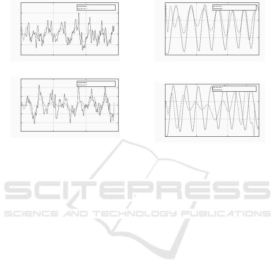
Figure 3 shows the results of applying the poly-

nomial adjustment method to both muscles, the VM

and the VL. Observe that the polynomial adjustment

curve follows the EMG signal trend even if it does

not reach the signal amplitude. As indicated before,

the polynomial obtained is of degree 20, which can

predict any signal peak. It is worth to remark that

a polynomial with a higher degree does not guaran-

tee better results but it implies a higher computational

cost. Other approaches may use lower degree polyno-

mials, e.g. (Earp et al., 2013) that obtains a 4th degree

polynomial, but the motion in that case is slow, while

here it can be either fast or slow.

To validate the polynomial adjustment method we

compare the post-processed signal with the NOTCH

signal obtained from the same experiment and at

the same time. Figure 4 shows the VM and the

VL muscles with the polynomial adjustment and

the validation signal, where we can see that the al-

gorithm takes approximately three seconds to follow

the NOTCH signal. It is worth to remark that the

highest peak on the Notch signal represents the sub-

ject’s muscle maximum-effort contraction. As a res-

ult, for the knee extension the angular position sig-

nal corresponds to the NOTCH output for the VM

ICINCO 2019 - 16th International Conference on Informatics in Control, Automation and Robotics

734

0 5 10 15

Time(s)

-1

-0.5

0.5

1.5

Normalized EMG signal (v/v)

Polynomial adjustment vastus medialis

EMG

Polynomial adjustment

(a) Knee angular position from the Polynomial ad-

justment vs. EMG signal on the vastus medialis

0 5 10 15

Time(s)

-1.5

-1

-0.5

0.5

1.5

Normalized EMG signal (v/v)

Polynomial adjustment vastus lateralis

EMG

Polynomial adjustment

(b) Knee angular position from the Polynomial

adjustment vs. EMG signal on the vastus lateralis

Figure 3: Knee angular position obtained from the Poly-

nomial adjustment method and EMG signal from the vastus

lateralis and the vastus medialis muscles.

muscle in time and amplitude, while for the ﬂexion

the polynomial adjustment follows the trend, but does

not reach the amplitude. The main reason for this is

that the VM and the VL are contracted mainly in the

knee extension. The mean correlation coefﬁcient is

mean

= 0.558, which indicates that half of the sig-

nal (the portion corresponding to the extension) is cor-

rectly predicted. Additionally, the VM muscle reveals

better results than the evaluation of the VL muscle.

The results of the application of the LWPR

method are shown in Figure 5. As presented in sec-

tion 2.2, each point of the joint angular position is

estimated from the EMG signal for each user. Figures

5(a) and 5(b) show the angular joint position obtained

from the application of the LWPR approach for the

VM muscle, and for the VL muscle respectively. In

the former case, the algorithm works properly after

2.5 s of execution. This means that the ﬁrst data, up

to 2.5 s are not valid and we do not consider them for

the validation. It can be seen that LWPR algorithm

tries to follow the maximum peaks of the signal for

both muscles, but it presents problems in following

the minimum values for the VL and the VM, differ-

ent from the polynomial approach that works better

in following both the minimum and maximum peaks.

Tables 1 and 2 show the correlation coefﬁcient

(CC) obtained when comparing the NOTCH signal

with the outputs of the algorithms after the signal

0 5 10 15

Time(s)

100

150

Degrees

Adjusted polynomial vs validation signal vastus medialis

100

150

EMG polynomial adjustment

Notch signal

(a) Knee angular position from the Polynomial ad-

justment vs. Validation signal on the vastus me-

dialis

0 5 10 15

Time(s)

100

150

Degrees

Adjusted polynomial vs validation signal vastus lateralis

100

150

EMG polynomial adjustment

Notch signal

(b) Knee angular position from the Polynomial ad-

justment vs. Validation signal on the vastus lat-

eralis

Figure 4: Knee angular position from the Polynomial

adjustment compared to the validation signal of NOTCH

sensors on the vastus lateralis and the vastus medialis

muscles.

post-processing. As a result, for the VM muscle,

mean

= 0.356 and CC

mean

= 0.558 for the LWPR

and the polynomial adjustment respectively. On the

other hand, for the VL muscle, CC

mean

= 0.3741 and

mean

= 0.500 for the LWPR and the polynomial ad-

justment respectively. These results can also be ob-

served in Figures 4(a), and 6(a) previously analyzed,

where the polynomial adjustment reaches better res-

ults than the LWPR method. The CC shows that the

approaches of each algorithm explain the knee exten-

sion, because the VM and VL muscles are mainly

contracted when the knee is extended. However, in

order to evaluate the total range of motion during the

knee ﬂexion-extension, it is necessary to use the sig-

nals obtained from other muscles such as the ham-

string. The VM EMG data allows to explain better the

joint angular position than the VL. This can be seen

comparing the CC, that in the ﬁrst case is of about

50% while in the latter is about 37%.

Finally, to evaluate the computational cost in

terms of the time required to ﬁnish the processing, we

tested the algorithms on an ASUS G5551VW with In-

tel Core i7-6700HQ processor, RAM of 16 GB and an

NVIDIA GeForce GTX 960M graphic card. The time

required by the LWPR method was 310.55 s, while

the time required for the polynomial adjustment was

Electromyography Signal Analysis to Obtain Knee Joint Angular Position

735

0 5 10 15

Time(s)

-1

-0.5

0.5

1.5

Normalized EMG signal (v/v)

Locally Weighted Projection Regression vastus medialis

EMG

LWPR

(a) Polynomial set in the VM: knee angular posi-

tion obtained from the LWPR method

0 5 10 15

Time(s)

-1.5

-1

-0.5

0.5

1.5

Normalized EMG signal (v/v)

Locally Weighted Projection Regression vastus lateralis

EMG

LWPR

(b) Polynomial set in VL: knee angular position

obtained from the LWPR method

Figure 5: Knee angular position from the LWPR method

and EMG signal from the vastus lateralis and the vastus me-

dialis muscles.

0.222 s. The former method spends more time be-

cause of the learning processes and the prediction of

the required parameters.

Table 1: Validation data on vastus medialis.

Vastus medialis

Metod CC

mean

Delay(s)

LWPR 0.356 -0.325

P adjustment 0.558 -0.114

Table 2: Validation data on vastus lateralis.

Vastus lateralis

Metod CC

mean

Delay(s)

LWPR 0.3741 -0.775

P adjustment 0.500 -0.74

5 CONCLUSION

We have presented an algorithm to determine the joint

angular positions from surface Electromyography

(EMG) measurements with the aim of using these

data for control systems of assistive devices. Two ap-

proaches have been explored, i.e. a polynomial ad-

justment method and a LWPR method. These meth-

ods allow a curve ﬁtting to obtain joint angular po-

sition from EMG. To validate the obtained curves,

we compared the data obtained from the curve ﬁt

with the measurements obtained with position sensors

0 5 10 15

Time

-100

100

200

Degrees

LWPR vs validation signal vastus medialis

100

150

LWPR

Notch signal

(a) Knee angular position obtained from the

LWPR vs. Validation signal on vastus medialis

0 5 10 15

Time

-100

100

200

Degrees

LWPR vs validation signal vastus lateralis

100

150

LWPR

Notch signal

(b) Knee angular position obtained from the

LWPR vs. Validation signal on vastus lateralis

Figure 6: Knee angular position obtained from the LWPR

method compared with the validation signal of the vastus

lateralis and the vastus medialis.

NOTCH. In order to obtain EMG data from the

ﬂexion-extension motion, an experiment was carried

out, in which 20 subjects participated. As a result, we

found that the polynomial adjustment method evalu-

ating the EMG signal over the vastus medialis muscle

reached a higher similarity compared to the NOTCH

sensor signal. This test allowed to obtain similar sig-

nals from the curve ﬁtting of the EMG data, compared

with the NOTCH sensor in the extension of the knee.

This results are coherent because the muscles from

which we obtained the EMG data (i.e. the vastus lat-

eralis and the vastus medialis) are the main muscles

involved in the knee extension. Future work will

be oriented to use signals from other muscles to ex-

plain completely the ﬂexion-extension range of mo-

tion. This analysis can be done using more EMG

sensors. We expect to use real time algorithms but

as a drawback the computational cost will be incre-

mented.

ACKNOWLEDGMENT

This work is funded by Universidad Militar Nueva

Granada- Vicerrectoría de Investigaciones, under re-

search grant for project PIC-ING-2679, entitled ’Cara-

cterización de señales de electromiografía dirigido al

control de sistemas de rehabilitación de rodilla’.

ICINCO 2019 - 16th International Conference on Informatics in Control, Automation and Robotics

736

REFERENCES

Ajoudani, A., Tsagarakis, N. G., and Bicchi, A. (2012).

Tele-impedance: Towards transferring human imped-

ance regulation skills to robots. In Robotics and Auto-

mation (ICRA), 2012 IEEE International Conference

on, pages 382–388. IEEE.

Akhtar, A. (2016). Estimation of distal arm joint angles

from EMG and shoulder orientation for transhumeral

prostheses. PhD thesis.

Altobelli, A., Bianchi, M., Catalano, M. G., Serio, A.,

Baud-Bovy, G., and Bicchi, A. (2015). An instru-

mented manipulandum for human grasping studies. In

Rehabilitation Robotics (ICORR), 2015 IEEE Interna-

tional Conference on, pages 169–174. IEEE.

Chen, J., Zhang, X., Cheng, Y., and Xi, N. (2018). Sur-

face emg based continuous estimation of human lower

limb joint angles by using deep belief networks. Bio-

medical Signal Processing and Control, 40:335–342.

Earp, J. E., Newton, R. U., Cormie, P., and Blazevich,

A. J. (2013). Knee angle-speciﬁc emg normaliza-

tion: The use of polynomial based emg-angle relation-

ships. Journal of Electromyography and Kinesiology,

23(1):238–244.

Ema, R., Wakahara, T., and Kawakami, Y. (2017). Effect of

hip joint angle on concentric knee extension torque.

Journal of Electromyography and Kinesiology.

Fang, C., Ajoudani, A., Bicchi, A., and Tsagarakis, N. G.

(2018). Online model based estimation of complete

joint stiffness of human arm. IEEE Robotics and Auto-

mation Letters, 3(1):84–91.

Freriks, B. and Hermens, H. (2000). European recommend-

ations for surface electromyography: results of the

SENIAM project. Roessingh Research and Develop-

ment.

Garabini, M., Della Santina, C., Bianchi, M., Catalano, M.,

Grioli, G., and Bicchi, A. (2017). Soft robots that

mimic the neuromusculoskeletal system. In Conver-

ging Clinical and Engineering Research on Neurore-

habilitation II, pages 259–263. Springer.

Huo, W., Mohammed, S., Moreno, J. C., and Amirat, Y.

(2016). Lower limb wearable robots for assistance

and rehabilitation: A state of the art. IEEE Systems

Journal, 10(3):1068–1081.

Ito, S., Inui, D., Tateoka, K., Matsushita, K., and Sa-

saki, M. (2015). Wrist angle estimation based on

bilinear model using electromyographic signals from

circularly-attached electrodes. In 2015 54th Annual

Conference of the Society of Instrument and Control

Engineers of Japan (SICE), pages 1167–1172.

Jensen, G. M. and Lorish, C. D. (1994). Promoting pa-

tient cooperation with exercise programs. linking re-

search, theory, and practice. Arthritis and Rheumat-

ism, 7:181–189.

Khan, K. M. and Scott, A. (2009). Mechanotherapy: how

physical therapists’ prescription of exercise promotes

tissue repair. British Journal of Sports Medicine,

43(4):247–252.

Koller-Hodac, A., Leonardo, D., Walpen, S., and Felder,

D. (2010). A novel robotic device for knee rehabili-

tation improved physical therapy through automated

process. In 2010 3rd IEEE RAS EMBS International

Conference on Biomedical Robotics and Biomechat-

ronics, pages 820–824.

Koller-Hodac, A., Leonardo, D., Walpen, S., and Felder, D.

(2011). Knee orthopaedic device how robotic tech-

nology can improve outcome in knee rehabilitation.

In 2011 IEEE International Conference on Rehabili-

tation Robotics, pages 1–6.

Li, H. and Cheng, L. (2017). Preliminary study on the

design and control of a pneumatically-actuated hand

rehabilitation device. In 2017 32nd Youth Academic

Annual Conference of Chinese Association of Auto-

mation (YAC), pages 860–865.

Mghames, S., Laghi, M., Santina, C. D., Garabini, M.,

Catalano, M., Grioli, G., and Bicchi, A. (2017).

Design, control and validation of the variable stiffness

exoskeleton ﬂexo. In 2017 International Conference

on Rehabilitation Robotics (ICORR), pages 539–546.

Pang, M. and Guo, S. (2013). A novel method for elbow

joint continuous prediction using emg and musculo-

skeletal model. In 2013 IEEE International Confer-

ence on Robotics and Biomimetics (ROBIO), pages

1240–1245.

Peng, W. (2008). Energy analysis method of computa-

tional complexity. In 2008 International Symposium

on Computer Science and Computational Technology,

volume 2, pages 682–685.

Ren, Y., Wu, Y., Yang, C., Xu, T., Harvey, R. L., and Zhang,

L. (2017). Developing a wearable ankle rehabilitation

robotic device for in-bed acute stroke rehabilitation.

IEEE Transactions on Neural Systems and Rehabili-

tation Engineering, 25(6):589–596.

Stegeman, D. and Hermens, H. (2007). Standards for suface

electromyography: The european project surface emg

for non-invasive assessment of muscles (seniam). 1.

Umivale, P. S. (2011). Patología de la rodilla: Guía de

manejo clínico.

Vijayakumar, S., D’Souza, A., and Schaal, S. (2006). In-

cremental online learning in high dimensions. Neural

computation, 17:2602–34.

Vijayakumar, S. and Schaal, S. (2000). Locally weighted

projection regression: An o(n) algorithm for incre-

mental real time learning in high dimensional spaces.

In Proceedings of the Seventeenth International Con-

ference on Machine Learning (ICML 2000), volume 1,

pages 288–293, Stanford, CA. clmc.

Wang, P., McGregor, A. H., Tow, A., Lim, H. B., Khang,

L. S., and Low, K. H. (2009). Rehabilitation control

strategies for a gait robot via emg evaluation. In 2009

IEEE International Conference on Rehabilitation Ro-

botics, pages 86–91.

Yap, H. K., , Nasrallah, F., Goh, J. C. H., and Yeow, R. C. H.

(2015). A soft exoskeleton for hand assistive and reha-

bilitation application using pneumatic actuators with

variable stiffness. In 2015 IEEE International Con-

ference on Robotics and Automation (ICRA), pages

4967–4972.

Electromyography Signal Analysis to Obtain Knee Joint Angular Position

737