
Water-resource Optimization Problem of Inland Waterways based on
Network Flows with Flow Transition Time and Time Varying
Characteristics
Eric Duviella
1,2
, Baya Hadid
1,2
and D
´
ebora C. C. S. Alves
1,2
1
Institut Mines Telecom Lille Douai, F-59000 Lille, France
2
Univ. Lille, Lille, France
Keywords:
Model Graph, Large Scale Systems, Optimization, Modelling, Water System.
Abstract:
Water-resource allocation planning is a well studied problem that aims at sharing water-resource to answer to
multi-objective management. For inland waterways, water-resource has to be balanced among the networks
to guaranty navigation conditions as a priority. Hydraulic devices such as locks and gates are used to transfer
volumes of water between the interconnected navigation reaches that composed the network. By considering
a large spatial scale with a low control time scale, transport delays have to be considered. Hence, network
flows with flow transition time and time varying characteristics is proposed to deal with transport delays and
modifications of the operating conditions over time. Network flows are then used for the optimization step.
The proposed model and optimization approach are illustrated by considering an inland waterway that is
composed of two navigation reaches.
1 INTRODUCTION
Hydrographical networks are large scale systems that
carry volumes of water. These systems have been de-
veloped over the time to meet human’ needs. They
have been equipped with dams to store the water, ex-
pansion areas to reduce flood impacts, gates to con-
trol water dispatching, and locks to allow navigation.
Whatever the hydrographical networks, the water-
resource has to be shared between usages. Hence
multi-objective management has to be performed
(Tchangani, 2017; Amigoni et al., 2015; Xiong et al.,
2018; He et al., 2018). This management requires
the definition and the solving of water-resource opti-
mization problems. In (Duviella et al., 2018), water-
resource allocation planing based on quadratic opti-
mization technique is proposed to guaranty the nav-
igation conditions and to study the resilience of the
waterways against extreme events. The requirement
of good extreme event prediction based on accurate
rainfall/runoff model is discussed in (Hadid and Du-
viella, 2018). Rainfall/runoff models are based on
offline and recursive/online parameter estimation of
data-driven linear and nonlinear models (Hadid et al.,
2018). In addition, a predictive optimization ap-
proach is proposed in (Alves et al., 2018) to improve
again the water management. These approaches are
based on an integrated model of inland waterways
and on a weighted dynamic generative network flow
that is introduced in (Fathabadi and Hosseini, 2010).
The management time corresponds to half of a day
implying that no transfer delays have been consid-
ered. Moreover, the arcs capacities and node sup-
plies/demands are functions of time. Based on these
assumptions, it is assumed that the transfer of water-
resource between two reaches is immediate between
two time steps. When the transfer delays have to be
considered in the optimization, the method requires
temporized flow networks or flow over time networks.
In (Ladeveze et al., 2010), a transportation network is
proposed to implement an algorithm leading to opti-
mal trajectories of a multi-objective short-term man-
agement of a dam-river system. A time expanded flow
network formalism is used in (Ayoub et al., 2018)
to consider available hydraulic data. A similar ex-
tended flow network is used in (Bencheikh et al.,
2017) to decrease the flood impacts thanks to the use
of flood expansion area with a real case-study located
in the south of France. The proposed transportation
networks are based on those described in (Kotnyek,
2003) that aim at considering the time for the flow to
pass the arcs, the storage capability for each node, the
time varying characteristics of the nodes and arcs, and
the concept of throughput in the dynamics of the flow
Duviella, E., Hadid, B. and Alves, D.
Water-resource Optimization Problem of Inland Waterways based on Network Flows with Flow Transition Time and Time Varying Characteristics.
DOI: 10.5220/0007924603030310
In Proceedings of the 16th International Conference on Informatics in Control, Automation and Robotics (ICINCO 2019), pages 303-310
ISBN: 978-989-758-380-3
Copyright
c
2019 by SCITEPRESS – Science and Technology Publications, Lda. All rights reserved
303

networks. The main objective is a well understanding
and representing of the dynamics of hydrographical
systems.
Flow network modeling is more dedicated to op-
timization applications. To this aim, a decomposition
of the hydrographical networks in conceptual mod-
els is required. In (Ladeveze et al., 2010; Ayoub
et al., 2018; Bencheikh et al., 2017; Duviella et al.,
2018), the nodes of the flow networks correspond to
reaches or parts of reach between hydraulic devices
such as gates, locks, hydraulic inputs, etc. A system-
atically decomposition approach has been proposed
in (Wolfs et al., 2015). It allows considering concep-
tual models based on virtual reservoirs. In this pa-
per, the decomposition of inland navigation reaches
is based on the Integrator Delay (ID) model (Schuur-
mans et al., 1999) to take into account the backwater
effect that characterizes these systems. Indeed, nav-
igation reaches, depending of their size, can be con-
sidered as tanks due to the presence of locks. More-
over, most of them are characterized by a very small
slope or no slope that increases the backwater effect
and some resonance phenomena (Segovia et al., 2017;
Horv
`
ath et al., 2015; Horv
´
ath et al., 2014). These
three contributions are dedicated to predictive control
of water level and not on water resource dispatching.
By considering a large spatial scale and a low con-
trol time scale, the modelling of inland waterways
with flow networks requires a priori flow transition
time, storage capability, time varying characteristics
and throughput dynamics. Based on these concepts, a
network flow with flow transition time and time vary-
ing characteristics is proposed. It is well suited to in-
land waterways and optimal water-resource allocation
planning.
The paper is organized as follows: Section II de-
scribes the inland waterways and the modelling ap-
proach based on ID model. The network flows with
flow transition time and time varying characteristics
are detailed in Section III. Section IV deals with the
optimization approach. Finally, a case-study is given
in Section V to illustrate the modeling and optimal
water-resource allocation steps.
2 INLAND WATERWAYS
2.1 Description and Management
Objectives
Inland waterways are large scale and complex sys-
tems that are used principally for navigation. They
are usually composed with interconnected Navigation
Reaches, denoted NR, and equipped with locks that
allow guaranteeing the navigation condition whatever
is the landform. Artificial canals have been built to
connect natural rivers and to permit navigation trans-
port.
The main management objective consists in guar-
anteeing the navigation conditions at each time all
along the year. An objective that is denoted Normal
Navigation Level (NNL) and a navigation rectangle
are defined for each NR. The navigation rectangle is
an interval around the NNL that is composed of a low
limit, the Low Navigation Level (LNL) and a high
limit, the High Navigation Level (HNL). The water-
resource management consists in allocating the avail-
able resource among the interconnected NR to keep
their water levels inside the defined navigation rect-
angle and closest as possible to the NNL. The main
disturbances are from the navigation demand i.e. the
ships crossing the locks. At each lock operation, a
big water volume goes from the upstream NR to the
downstream one. Moreover, because inland water-
ways are strongly connected with other natural rivers,
and inside watersheds, they are also affected by cli-
matic events.
The water-resource allocation is performed thanks
to the controlled gates by taking into account the con-
figuration of the waterways. Depending on the control
time scale, the transfer delay, i.e. the required time a
volume of water travels from an upstream to a down-
stream point, must be considered. Otherwise, an order
can be sent to a controlled gate before that the water
volume arrives this gate leading to deficit of water.
2.2 Integrated Model
A first model entitled integrated model is proposed
to well represent the waterways configuration and the
possible interactions with naturals rivers or other hy-
draulic systems that are not considered by the water-
resource allocation planning (Duviella et al., 2018).
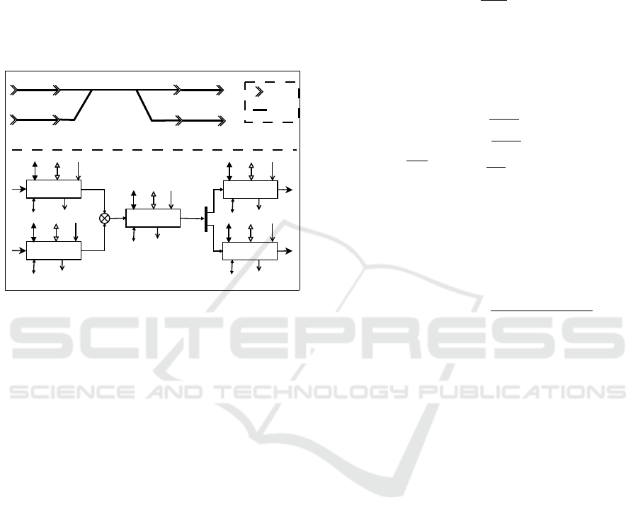
Fig. 1.a shows an example of a waterway composed
with five NR and the two elementary configurations;
a tributary and a distributary. The corresponding inte-
grated model is depicted in Fig.1.b, with:
• V
s,c
i
and respectively V
e,c
i
, the controlled volumes
from one or several upstream NR that supply and
(resp.) empty the NR
i
(s: supply, e: empty, c:
controlled),
• V
c
i
the controlled volumes from water intakes that
can supply or empty NR
i
. These volumes are
signed; positive if NR
i
is supplied, negative oth-
erwise,
• V
s,p
i
and (resp.) V
e,p
i
the controlled volumes from
ICINCO 2019 - 16th International Conference on Informatics in Control, Automation and Robotics
304
pump that can supply and (resp.) empty the NR
i
,
denoted (p: pumped),
• V
u
i
the uncontrolled volumes from natural rivers,
rainfall-runoff, Human uses (u: uncontrolled).
These volumes are signed depending on their con-
tribution to the volume V
i
(k) in NR
i
.
• V
g,u
i
the uncontrolled volumes from exchanges
with groundwater (g: groundwater), that can be
associated to V
u
i
.
(a)
Lock
NR
NR
i-2
NR
i-1
NR
i
NR
i+1
NR
i+2
(b)
NR
i
NR
i-2
NR
i-1
NR
i+1
NR
i+2
V
i
s,c
V
i
e,c
V
i
u
V
i
c
V
i
g,u
V
i-2
s,c
V
i-2
e,c
V
i-2
u
V
i-2
c
V
i-2
g,u
V
i-1
s,c
V
i-1
e,c
V
i-1
u
V
i-1
c
V
i-1
g,u
V
i+1
s,c
V
i+1
e,c
V
i+1
u
V
i+1
c
V
i+1
g,u
V
i+2
s,c
V
i+2
e,c
V
i+2
u
V
i+2
c
V
i+2
g,u
+
+
V
i-2
s,p
V
i-2
e,p
V
i-1
s,p
V
i-1
e,p
V
i
s,p
V
i
e,p
V
i+1
s,p
V
i+1
e,p
V
i+2
s,p
V
i+2
e,p
Figure 1: a. Inland waterways, b. corresponding integrated
model.
The dynamics of the reach NR
i
with a discrete
sample time T
s
is given by:
V
i
(k) = V
i
(k −1) +V
s,c
i
(k) −V
e,c
i
(k) +V
c
i
(k)
+V
s,p
i
(k) −V
e,p
i
(k) +V
u
i
(k) +V
g,u
i
(k),
(1)
where k corresponds to the current period of time and
k −1 the last one.
This model is well suited for the representation
of waterways where no transfer delay has to be taken
into account. Otherwise, it is necessary to decompose
the NR in conceptual NR according to the transfer de-
lays and the control sample time.
2.3 Conceptual Navigation Reach
Model
The conceptual navigation reach model is designed
based on the Integrator Delay model (Schuurmans
et al., 1999). The ID model aims at linking the dis-
charges that supply/empty a reach to water levels of
the reach, at least on the two points that correspond to
the boundaries of the reach. It can be expressed as:
y(1,s)
...
y( j,s)
...
y(n,s)
=
p
11
(s) p
12
(s) ... p
1m
(s)
... ... ... ...
p
j1
(s) p
j2
(s) ... p
jm
(s)
... ... ... ...
p
n1
(s) p
n2
(s) ... p
nm
(s)
q(1,s)
...
q(i,s)
...
q(m,s)
(2)
where y( j,s) is the j
th
water level, j ∈1 : n, q(i,s) the
i
th
discharge input/output, i ∈ 1 : m, with n the num-
ber of measurement points and m the number of dis-
charge points. p
ji
(s) is a term of the ID model that is
expressed as:
p
ji
(s) =
1
A
ji
.s
e
−τ
ji
.s
(3)
with A
ji
the integrator gain that corresponds to the
area of the reach A = L ∗W , with L the length and
W the width of the reach. The transfer time delays
τ
ji
, (resp.) τ
i j
, between the points j and i that are L
ji
meters apart, with j upstream to i, are expressed by:
(
τ
ji
=
L
ji
C
0
−V
0
,
τ
i j
=
L
ji
C
0
+V
0
(4)
with C
0
=
√
g.D and V
0
=
Q
0
W.D
, where g is the gravity
and D the depth of the reach for the nominal discharge
Q
0
.
Based on this model and considering a discrete
sample time T
s
, it is possible to represent the dynam-
ics of each part of the reach with a virtual tank of area
A that is supplied and emptied with the delayed dis-
charges. Thus:
y
j
(k) = y
j
(k −1) +
∑
m
i=1
q
i
(k −T
ji
).T
s
A
(5)
with q
i
(k) a signed discharge and T
ji
= bτ
ji
/T
s
c,
where bc provides the floor integer number.
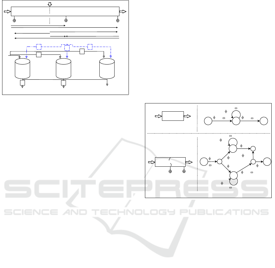
Fig.2.a depicts a schematic view of a NR with
multiple inputs/outputs (discharges Q
i
) and measure-
ment points (levels Y
j
), and the corresponding delays
between these points. Note that the delays T
ji
when
i is located in the same place than j are not shown
because they are equal to 0. The corresponding con-
ceptual model is shown in Fig.2.b, where a tank is as-
sociated to each measurement point. The area of the
tanks is the same. These tanks are supplied/emptied
with delayed discharges according to the configura-
tion of the waterway. This conceptual model is then
used to design the network flows.
3 NETWORK FLOWS
The definition and the description of static network
flows are proposed in (Ahuja et al., 1993). In (Kot-
nyek, 2003), a state of the art of dynamic network
flows is given. It aims at describing a formalism of
dynamic network flows able to take into account flow
time, storage capability, time varying characteristics,
and the concept of throughput. All these properties
are required to model inland waterways thanks to net-
work flows. Hence, the proposed network flow is de-
fined on a direct graph G = (N, E,B,T,Ω,Φ), with:
Water-resource Optimization Problem of Inland Waterways based on Network Flows with Flow Transition Time and Time Varying
Characteristics
305
Y
1
Y
j
Y
n
Q
1
Q
m
T
1n
T
mj
T
in
T
i1
T
m1
T
1j
Q
i
(a)
Q
1
Q
m
T
1n
T
1j
T
mj
T
m1
Y
1
Y
j
Y
n
T
in
T
i1
Q
i
(b)
T
ij
T
ij
Figure 2: a. schematic view of a NR with transfer delays, b.
corresponding conceptual model.
• the nodes N = N
i
∪N
c
∪N
T
∪O∪S, with O the su-
persource, S the supersink that gather respectively
all the sources and all the sinks, N
i
the set of nodes
that corresponds to the NR or parts of NR, N
c
the
set of conceptual nodes, and N
T
the set of tempo-
rized nodes,
• the arcs E = E
i
∪E
c
∪E
T
∪E
d
, with E
i
the set of
arcs between NR, source O and sink S, E
c
the set
of conceptual arcs, E
T
the set of temporized arcs,
and E
d
the set of arcs starting from and entering
in the same NR allowing the modelling of the ca-
pacity of the nodes N
i
,
• the boundaries B = B
e
∪B
d
are composed of a
lower and a higher limits, l
i j
(k) and u
i j
(k) respec-
tively , with B
e
the set of boundaries associated to
arcs E
i
, and B
d
the set of boundaries associated to
arcs E
d
,
• the transfer delays T that are associated to the set
of arcs E
T
,
• the weights Ω = Ω
i
∪Ω
d
that are associated to the
set of arcs E
i
∪E
d
, respectively,
• the flows Φ = Φ
i
∪Φ
c
∪Φ
T
∪Φ
d
that are trans-
ferred by the set of arcs E.
The limits and weights can change over the time.
They are expressed according to time k. Hence, the
network flow has time varying characteristics.
For an inland waterway that is composed of one
NR where the maximum transfer delay is lower than
the sample time, i.e. maxbτ
ji
/T
s
c = 0, (see Fig.3.a),
the corresponding network flow (see Fig.3.b) is de-
fined as:
• N = N
i
∪O ∪S, with N
i
= {1}, N
T
= ∅ and N
c
=
∅,
• E = E
i
∪E
d
, with E
i
= {e
O1
, e
1S
}, E
d
= {e
11
}
where e
i j
is the arc between nodes i and j, E
c
= ∅
and E
T
= ∅,
• B = B
e
∪ B
d
, with B
e
=
{[l
O1
(k), u
O1
(k)], [l
1S
(k), u
1S
(k)]} and
B
d
= {[l
11
(k), u
11
(k)]}, where l
i j
(k) (resp.
u
i j
(k)) is the lower (higher) limit of the flow that
passes trough the arc e
i j
,
• T = ∅,
• Ω = Ω
i
∪Ω
d
, with Ω
i
= {w
O1
(k), w
1S
(k)}, Ω
d
=
{w
11
(k)},
• Φ = Φ
i
∪Φ
d
, with Φ = {φ
O1
(k), φ
1S
(k)}, Φ
d
=
{φ
11
(k)}, where φ
i j
(k) is the flow that passes
through the arc e
i j
at time k, Φ
c
= ∅ and Φ
T
= ∅.
Q
1
Q
2
NR
1
(a)
(b)
Q
1
Q
2
NR
1
Y
1
Y
2
O S
[l (k), u (k)]
(k)
(k)
1
a
1
a
1
a
1
a
1
a
1
a
1
a
1
a
1
a
[l (k), u (k)]
(k)
(k)
1
b
b
1
b
1
b
1
b
1
b
1
b
1
b
1
b
1
C
(k)
O
a
1
(k-T )
O
a
1
(k)
a
1
O
[l (k), u (k)]
a
1
a
1O O
O 1 S
[l (k), u (k)]
11
11
11
(k)
O1
(k)
O1
(k)
11
(k)
1S
(k)
1S
(k)
[l (k), u (k)]
1S
1S
[l (k), u (k)]
O1
O1
12
(k)
O
1
a
(k)
S
1
b
(k)
S
1
b
(k-T )
S
1
b
21
T
1
T
2
(k)
[l (k), u (k)]
S
1
b
S
1
b
S
1
b
(k)
a
1 C
(c)
(d)
1
a
1
b
Figure 3: a. NR without consideration of time delay, b.
corresponding network flows, c) NR with consideration of
time delay, d) corresponding network flows.
When the maximum transfer delays is higher than
the sample time (see Fig.3.c), i.e. maxbτ
ji
/T
s
c ≥ 1,
the corresponding network flow (see Fig.3.d) is de-
fined as:
• N = N
i
∪N
c
∪N
T
∪O∪S, with N
i
= {1a, 1b}, N
c
=
{C}, N
T
= {T
1
, T
2
},
• E = E
i
∪E
c
∪E
T
∪E
d
, with E
i
= {e
OT
1
, e
1
b
T
2
},
E
d
= {e
1
a
1
a
, e
1
b
1
b
} and E
c
= {e
1
a
C
}, E
T
=
{e
T
1
1
a
, e
T
1
1
b
, e
T
2
C
, e
T
2
S
},
• B = B
e
∪ B
d
, with B
e
=
{[l
O1
a
(k), u
O1
a
(k)], [l
1
b
S
(k), u
1
b
S
(k)]} and
B
d
= {[l
1
a
1
a
(k), u
1
a
1
a
(k)], [l
1
b
1
b
(k), u
1
b
1
b
(k)]},
where l
i j
(k) (resp. u
i j
(k)) is the lower (higher)
limit of the flow that passes trough the arc e
i j
, at
time k,
• T = {T
12
, T
21
},
• Ω = Ω
i
∪ Ω
d
, with Ω
i
= {w
O1
a
(k), w
1
b
S
(k)},
Ω
d
= {w
1
a
1
a
(k), w
1
b
1
b
(k)},
• Φ = Φ
i
∪ Φ
C
∪ Φ
T
∪ Φ
d
, with Φ
i
=
{φ
O1
a
(k), φ
1
b
S
(k)} and Φ
C
= {φ
1
a
C
(k)},
ICINCO 2019 - 16th International Conference on Informatics in Control, Automation and Robotics
306
Φ
d
= {φ
1
a
1
a
(k), φ
1
b
1
b
(k)} and Φ
T
=
{φ
O1
a
(k), φ
1
b
S
(k), φ
O1
a
(k −T
12
), φ
1
b
S
(k −T
21
)}.
The set of nodes N
i
verifies the Kirchhoff’s law
such as:
∑
j∈E
+
N
i
φ
e
j
(k) −
∑
j∈E
−
N
i
φ
e
j
(k) = 0 (6)
with E
+
N
i
and E
−
N
i
(resp.), the set of arcs entering, out-
going (resp.) the node N
i
, and φ
e
j
the flow associated
to the arc e
j
.
The set of temporized nodes N
T
do not verify the
conservation rule as it is specified in (Kotnyek, 2003).
It allows associating a transfer delay to each of the
flow outgoing the temporized node:
φ
e
j
(k) = φ
e
N
T
(k −T
j
) (7)
with j ∈ E
−
N
T
, the set of arcs outgoing the node N
T
,
e
N
T
the arc that enters the node N
T
, and T
j
the transfer
delay that is associated to the outgoing arc e
j
.
The set of conceptual node N
C
verifies a conser-
vation law between the flow on the arc outgoing the
nodes N
i
(e
−
N
i
) and the flow on the arc outgoing the
nodes N
T
(e
−
N
T
), defined as:
φ
e
−
N
i
(k) = φ
e
−
N
T
(k −T
j
) (8)
The optimization of dynamic network flows leads
to NP-hard problem as it is stated in (Skutella, 2009).
To overcome this problem, a formalism of extended
network flow has been proposed in (Fulkerson, 1966)
and used in (Ladeveze et al., 2010; Bencheikh et al.,
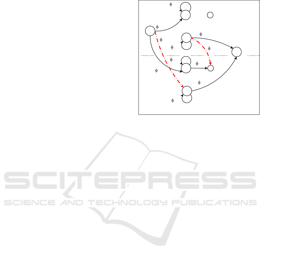
2017). The network flows in Fig. 3.d is represented
in Fig.4 by considering T
12
= T
21
= 1 and two step
times from k = 1 to k = 2. The dashed red arcs rep-
resent the temporized flows. Depending of the value
of maxbτ
ji
/T
s
c, a throughput is defined and the opti-
mization can be done for each of it. In this example,
this throughput is equal to 2. Finally, some optimiza-
tion approaches can be applied.
4 WATER-RESOURCE
ALLOCATION PLANNING
The allocation planning consists in dispatching the
water-resource among the waterways by keeping the
volume inside each NR close to their objective (Du-
viella et al., 2018). These objectives are defined in
relative value with the volumes that correspond to the
NNL. Thus, a capacity of a NR equal to 0 corresponds
to the NNL. The capacity boundaries are defined with
the LNL and HNL, with negative and positive bound-
aries. They are associated with the boundaries B
d
.
O
(1)
1
a
1
a
1
a
(1)
1
b
b
1
b
1
C
(1)
O
a
1
(1)
S
1
b
(2)
1
a
1
a
1
a
(2)
1
b
b
1
b
1
C
(2)
S
1
b
(2)
O
a
1
S
(1)
O
a
1
(2)
a
1 C
(1)
S
1
b
k=1
k=2
Figure 4: Time representation of the network flows depicted
in Fig.3.d.
The dynamics for inland waterways are defined ac-
cording the relations (7-9) following the configuration
of the network.
The water-resource allocation planning is per-
formed according to an optimization approach that
consists in minimizing the absolute value of the NR’s
capacity by exchanging water through the arcs be-
tween the source and the sink. In order to minimize
the water volume inside the NR, the weights Ω
d
that
are associated to the arcs E
d
have to be big. Other
weights Ω
i
that are associated to the arcs E
i
are tuned
according to the priority of the paths from a part of the
network to another one. Thus, the objective function
can be defined as:
J
V
=
∑
N
i
∈E
i
|
∑
j∈E
+
N
i
ω
j
(k)φ
e
j
(k)−
∑
j∈E
−
N
i
ω
j
(k)φ
e
j
(k)| (9)
by considering the constraints given by relation (6),
the boundaries B, and the transfer delays T . That
means that the exchanges of water volumes between
each NR or part of NR have to be balanced between
the entering and outgoing flows at each step time k.
For the waterway where the maximum transfer de-
lays is lower than the sample time (see Fig. 3.a), the
objective function to minimize is defined as:
J
V
= |ω
O1
(k)φ
O1
(k) +ω
11
(k)φ
11
(k) −ω
1S
(k)φ
1S
(k)|
(10)
with:
φ
O1
(k) +φ
11
(k) −φ
1S
(k) = 0,
φ
O1
(k) ∈ [l
O1
(k), u
O1
(k)],
φ
1S
(k) ∈ [l
1S
(k), u
1S
(k)],
φ
11
(k) ∈ [l
11
(k), u
11
(k)],
(11)
where ω
11
(k) ω
O1
(k) and ω
11
(k) ω
1S
(k) .
Water-resource Optimization Problem of Inland Waterways based on Network Flows with Flow Transition Time and Time Varying
Characteristics
307
For the waterway where the maximum transfer de-
lays is higher than the sample time (see Fig. 3.c),
the objective function to minimize has to be defined
by considering a throughput that is computed accord-
ing to the maximum transfer delay, i.e. from k to
k + maxbτ
ji
/T
s
c. In this case, by considering T
21
≥
T
12
, it is defined as:
J
V
= |ω
O1
a
(k)φ
O1
a
(k) +ω
1
a
1
a
(k)φ
1
a
1
a
(k)−
ω
1
b
S
(k −T
21
)φ
1
b
S
(k −T
21
)|+
|ω
O1
a
(k −T
12
)φ
O1
a
(k) +ω
1
b
1
b
(k)φ
1
b
1
b
(k)−
ω
1
b
S
(k)φ
1
b
S
(k)|+
...
|ω
O1
a
(k +T
21
)φ
O1
a
(k +T
21
)+
ω
1
a
1
a
(k +T
21
)φ
1
a
1
a
(k +T
21
)−
ω
1
b
S
(k +T
21
−1)φ
1
b
S
(k +T
21
−1)|+
|ω
O1
a
(k +T
21
−1)φ
O1
a
(k +T
21
)+
ω
1
b
1
b
(k +T
21
)φ
1
b
1
b
(k +T
21
)−
ω
1
b
S
(k +T
21
)φ
1
b
S
(k +T
21
)|
(12)
with, for k
0
∈ {k : k + T
21
}:
φ
O1
a
(k
0
) + φ
1
a
1
a
(k
0
) −φ
1
b
S
(k
0
−T
21
) = 0,
φ
O1
a
(k
0
−T
12
) + φ
1
b
1
b
(k
0
) −φ
1
b
S
(k
0
) = 0,
φ
O1
a
(k
0
) ∈ [l
O1
a
(k
0
), u
O1
a
(k
0
)],
φ
1
b
S
(k
0
) ∈ [l
1
b
S
(k
0
), u
1
b
S
(k
0
)],
φ
1
a
1
a
(k
0
) ∈ [l
1
a
1
a
(k
0
), u
1
a
1
a
(k
0
)],
(13)
where ω
1
a
1
a
(k
0
) ω
O1
a
(k
0
), ω
1
a
1
a
(k
0
) ω
1
b
S
(k
0
),
ω
1
b
1
b
(k
0
) ω
O1
a
(k
0
), ω
1
b
1
b
(k
0
) ω
1
b
S
(k
0
).
The optimization approach can be based on Con-
straints Satisfaction Problems (CSP) (Nouasse et al.,
2016b), on minimum cost problem (Kotnyek, 2003),
on linear programming (Nouasse et al., 2016a) or on
quadratic programming (Duviella et al., 2018). In this
paper, a linear programming approach based on the
Matlab function linprog
1
is used.
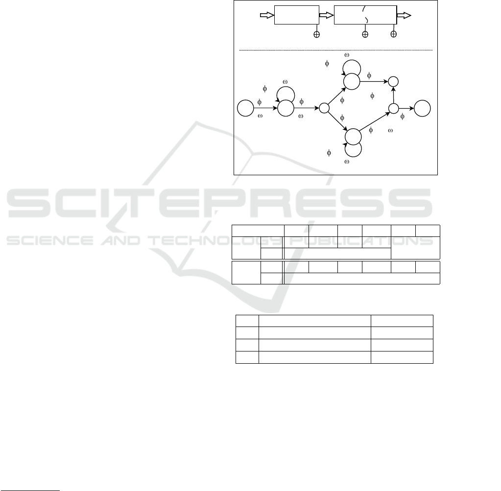
5 CASE-STUDY
The considered inland waterways is composed with
two NR as it is schematized in Fig. 5.a. The lengths of
the NR are L
NR
1
= 5 km, L
NR
2
= 20 km, with the same
width W = 20 m, nominal discharge Q
0
= 1 m
3
/s, and
depth D = 2.2 [m]. The parameters of the ID models
for both NR are identified (see Table 1). The sample
time is T
s
= 30 min. Thus, according to the transfer
delays, only NR
2
is decomposed in two parts. Fig.
5.b depicts the network flows associated to the case-
study. Hydraulic devices like locks and gates supply
and empty the NR. Their characteristics are given in
1
https://www.mathworks.com/help/optim/ug/linprog
.html
Table 2. The locks are activated for navigation and a
lock operation corresponds to a transfer of water vol-
ume between two NR. The duration of a lock opera-
tion is equal to 15 min. The gates can be controlled
inside the proposed intervals. Two periods of man-
agement are considered for the gate downstream NR
2
:
during 6 hours it can be controlled on the operating
range [0;5], the next 6 hours between [0; 10] [m
3
/s].
Q
1
Q
2
NR
1
(a)
(b)
Q
3
NR
2
Y
2
Y
3
S
[l (k), u (k)]
(k)
(k)
2
a
2
a
2
a
2
a
2
a
2
a
2
a
2
a
2
a
[l (k), u (k)]
(k)
(k)
2
b
b
2
b
2
b
2
b
2
C
(k-T )
12
a
O 1
[l (k), u (k)]
11
11
11
(k)
O1
(k)
O1
(k)
11
(k)
12
(k)
12
(k)
[l (k), u (k)]
12
12
[l (k), u (k)]
O1
O1
12
(k)
12
a
(k)
S
2
b
(k)
S
2
b
(k-T )
S
2
b
21
T
1
T
2
(k)
[l (k), u (k)]
S
2
b
S
2
b
S
2
b
(k)
a
2
C
2
a
2
b
Y
1
a
a
a a
b
2
b
2
b
2
b
2
Figure 5: a. Inland waterways composed with two NR, b.
network flows model.
Table 1: ID model parameters - τ [min].
P
11
P
12
P
21
P
22
P
31
P
32
NR
1
τ
i j
0 −18 17 0
A 100,000
NR
2
τ
i j
0 −71 35 −36 70 0
A 400,000
Table 2: Characteristics of the inputs/outputs of the NR.
Lock during 15 min Gate [m
3
/s]
Q
1
15,000 m
3
→ 16.66 m
3
/s -
Q
2
6,000 m
3
→ 6.66 m
3
/s [0; 10]
Q
3
7,000 m
3
→ 7.77 m
3
/s [0;(5 −10)
∗
]
The weights are tune such as ω
11
(k) = ω
2
a
2
a
(k) =
ω
2
b
2
b
(k) = 1,000 and ω
O1
(k) = ω
12
a
(k) = ω
2
b
S
(k) =
1, with the objective to minimize the water that is
stored inside the NR. Finally, according to the ID pa-
rameters, T
12
= T
21
= 2 T
s
.
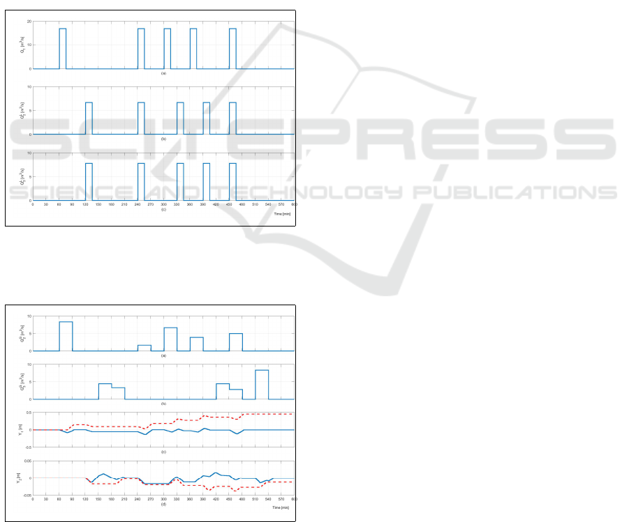
The lock operations over the future time horizon
2T
s
are supposed to be known and depicted in Fig.
6. The discharge Q
1
is the equivalent discharge due
to the lock operation upstream NR
1
during 15 min.
The discharges Q
L
2
and Q
L
3
come from the lock op-
erations upstream and downstream NR
2
(L for lock).
This knowledge allows the optimization of the crite-
ICINCO 2019 - 16th International Conference on Informatics in Control, Automation and Robotics
308
rion J
V
on horizon 2T
s
according to relation (9) and
the constraints given by relation (6).
A model of the considered inland waterway has
been implemented with Simulink/Matlab. The opti-
mization approach that is based on the linprog func-
tion is implemented with a matlab function. The sim-
ulation results are depicted in Fig. 7 with the con-
trolled discharges at the gates upstream and down-
stream NR
2
, i.e. Q
G
2
and Q
G
3
respectively (G for gate).
The resulting levels downstream NR
1
and NR
2
are de-
picted in Fig. 7.c and Fig. 7.d respectively. When no
optimization strategy is used, the simulation results
lead to the results depicted in dashed red line in Fig.
7.c and Fig. 7.d. These results are improved when the
proposed optimization approach is used as it is shown
in continuous blue line in Fig. 7.c and Fig. 7.d. The
maximum gap from the objective levels is lower when
the proposed approach is used.
Figure 6: a. The discharge due to the lock operations up-
stream NR
1
, b. the discharge due to the lock operations
upstream NR
2
, c. the discharge due to the lock operations
downstream NR
2
.
Figure 7: a. The controlled discharge upstream NR
1
, b. the
controlled discharge downstream NR
2
, c. the water level
downstream NR
1
, d. the water level downstream NR
2
.
6 CONCLUSIONS
In this paper a network flows with flow transition time
and time varying characteristics formalism is pro-
posed to deal with water-resource optimization of in-
land waterways. This formalism is based on the graph
theory. The design of the network flows is achieved
thanks to the ID model allowing the determination
of transfer delays. Then, an optimization approach
based on a linear programming is used. The proposed
approach is illustrated by considering an academical
case-study that consists in a two navigation reaches.
The main objective is to deal with time delays and
time varying characteristics. Future works will aim
at adapting and applying this approach on real sys-
tems with outlets to the sea that require time varying
characteristics to deal with the tide effect. Another
perspective will be the comparison of this approach
with MPC.
REFERENCES
Ahuja, R.-K., Magnanti, T.-K., and Orlin, J.-B. (1993).
Network flows - Theory, algorithms and applications.
New Jersey.
Alves, D. C. S., Duviella, E., and Doniec, A. (2018). Im-
provement of water resource allocation planning of in-
land waterways based on predictive optimization ap-
proach. In ICINCO, Porto, Portugal.
Amigoni, F., Castelletti, A., and Giuliani, M. (2015).
Modeling the management of water resources sys-
tems using multi-objective dcops. In Proceedings
of the 2015 International Conference on Autonomous
Agents and Multiagent Systems, AAMAS ’15, pages
821–829, Richland, SC. International Foundation for
Autonomous Agents and Multiagent Systems.
Ayoub, T., Ladeveze, D., Chiron, P., and Archim
`
ede,
B. (2018). Reconstruction of hydrometric data us-
ing a network optimization model. HIC conference,
Palermo, July 1st-6th.
Bencheikh, G., Tahiri, A., Chiron, P., Archimede, B.,
and Martignac, F. (2017). A flood decrease strategy
based on flow network coupled with a hydraulic sim-
ulation software 11this work was partially supported
by the urban community of le grand tarbes. IFAC-
PapersOnLine, 50(1):3171 – 3176. 20th IFAC World
Congress.
Duviella, E., Doniec, A., and Nouasse, H. (2018). Adap-
tive water-resource allocation planning of inland wa-
terways in the context of global change. Jour-
nal of Water Resources Planning and Management,
144(9):04018059.
Fathabadi, H. S. and Hosseini, S. A. (2010). Maximum flow
problem on dynamic generative network flows with
time-varying bounds. Applied Mathematical Mod-
elling, 34(8):2136 – 2147.
Water-resource Optimization Problem of Inland Waterways based on Network Flows with Flow Transition Time and Time Varying
Characteristics
309

Fulkerson, D. (1966). Flow networks and combinatorial op-
erations research. In American mathematical monthly,
volume 73.
Hadid, B. and Duviella, E. (2018). Water asset man-
agement strategy based on predictive rainfall/runoff
model to optimize the evacuation of water to the sea.
In ICINCO, Porto, Portugal.
Hadid, B., Duviella, E., and Lecoeuche, S. (2018). Im-
provement of a predictive data-driven model for
rainfall-runoff global characterization of aa river. cited
By 0.
He, Y., Chen, X., Sheng, Z., Lin, K., and Gui, F. (2018).
Water allocation under the constraint of total water-
use quota: a case from dongjiang river basin, south
china. Hydrological Sciences Journal, 63(1):154–167.
Horv
´
ath, K., Duviella, E., Petreczky, M., Rajaoarisoa, L.,
and Chuquet, K. (2014). Model predictive control of
water levels in a navigation canal affected by reso-
nance waves. In HIC 2014, 11th International Con-
ference on Hydroinformatics, New York.
Horv
`
ath, K., Rajaoarisoa, L., Duviella, E., Blesa, J., Pe-
treczky, M., and Chuquet, K. (2015). Enhancing in-
land navigation by model predictive control of water
level – the Cuinchy-Fontinettes case. Transport of Wa-
ter versus Transport over Water - Exploring the dy-
namic interplay between transport and water - Carlos
Ocampo-Martinez, Rudy Engenborn (eds).
Kotnyek, B. (2003). An annotated overview of dynamic
network flows. INRIA Report n. 4936.
Ladeveze, D., Charbonnaud, P., and Archim
`
ede, B. (2010).
Multi-objective management of multi-resource hy-
drographical systems. IFAC Proceedings Volumes,
43(8):585 – 590. 12th IFAC Symposium on Large
Scale Systems: Theory and Applications.
Nouasse, H., Doniec, A., Duviella, E., and Chuquet, K.
(2016a). Efficient management of inland navigation
reaches equipped with lift pumps in a climate change
context. 4
th
IAHR Europe Congress, Liege, Belgium
27-29 July.
Nouasse, H., Doniec, A., Lozenguez, G., Duviella, E., Chi-
ron, P., Archim
`
ede, B., and Chuquet, K. (2016b). Con-
straint satisfaction problem based on flow transport
graph to study the resilience of inland navigation net-
works in a climate change context. IFAC Conference
MIM, Troyes, France, 28-30 June.
Schuurmans, J., Clemmens, A. J., Dijkstra, S., Hof, A.,
and Brouwer, R. (1999). Modeling of irrigation and
drainage canals for controller design. Journal of irri-
gation and drainage engineering, 125(6):338–344.
Segovia, P., Rajaoarisoa, L., Nejjari, F., Puig, V., and Du-
viella, E. (2017). Decentralized control of inland nav-
igation networks with distributaries: application to
navigation canals in the north of France. ACC’17,
Seattle, WA, USA, May 24–26.
Skutella, M. (2009). An introduction to network flows over
time. In Research Trends in Combinatorial Optimiza-
tion, pages 451–482. Springer-Verlag.
Tchangani, A. P. (2017). Sustainable management of natu-
ral resource using bipolar analysis. application to wa-
ter resource sharing. IFAC-PapersOnLine, 50(1):3177
– 3182. 20th IFAC World Congress.
Wolfs, V., Meert, P., and Willems, P. (2015). Modular con-
ceptual modelling approach and software for river hy-
draulic simulations. Environmental Modelling & Soft-
ware, 71:60 – 77.
Xiong, W., Li, Y., Zhang, W., Ye, Q., Zhang, S., and
Hou, X. (2018). Integrated multi-objective optimiza-
tion framework for urban water supply systems un-
der alternative climates and future policy. Journal of
Cleaner Production, 195:640 – 650.
ICINCO 2019 - 16th International Conference on Informatics in Control, Automation and Robotics
310
