Middle Point Reduction of the Chain-recurrent Set

Carlos Arg

aez

1 a

, Peter Giesl

2 b

and Sigurdur Freyr Hafstein

1 c

Science Institute, University of Iceland, Dunhagi 5, 107 Reykjav

ık, Iceland

Department of Mathematics, University of Sussex, Falmer, BN1 9QH, U.K.

Keywords:

Lyapunov Functions, Chain-recurrent Set, Programming, Algorithm, Mathematics, Dynamical Systems.

Abstract:

Describing dynamical systems requires capability to isolate periodic behaviour. In Lyapunov’s theory, the

qualitative behaviour of a dynamical system given by a differential equation can be described by a scalar

function that decreases along solutions: the Complete Lyapunov Function. The chain-recurrent set will pro-

duce constant values of an associated complete Lyapunov function and zero values of its orbital derivative.

Recently, we have managed to isolate the chain-recurrent set of different dynamical systems in 2- and 3- di-

mensions. An overestimation, however, is always obtained. In this paper, we present a method to reduce such

overestimation based on geometrical middle points for 2-dimensional systems.

1 INTRODUCTION

The study of dynamical systems offers different

methodologies to approach time-evolving phenomena

expressed as ordinary differential equations. Several

disciplines ﬁnd in its semantics a powerful descriptive

language and in its results, useful tools to obtain solu-

tions. From a geometrical point of view, a dynam-

ical system describes the time-evolution of a point

in a state-space or geometrical manifold. Practically,

time-evolving phenomena can often be described as

a time-autonomous system of differential equations

given by the expression (1),

x = f(x), (1)

where x ∈ R

and n ∈ N. Furthermore, while seen

as function of its components, f : R

→ R

is a vec-

tor ﬁeld while

x represents the derivative against time.

Systems like (1), in which f(x) does not explicitly de-

pend on the time t, are called autonomous. However,

the solutions to (1) lead to time-dependent solutions

unless f(x) is identically zero.

The methodology to study and describe the be-

haviour of dynamical systems can vary. Since an ana-

lytical solution is only available in the simplest cases,

one could attempt to solve numerically the differen-

tial equation system (1) for a large collection of ini-

https://orcid.org/0000-0002-0455-8015

https://orcid.org/0000-0003-1421-6980

https://orcid.org/0000-0003-0073-2765

tial conditions. That would indeed describe the sys-

tem but only under a copious effort and would require

to ﬁnd a solution curve S

ξ, deﬁned as S

ξ := x(t) for

numerous initial condition x(0) = ξ ∈ R

Computing the invariant manifolds which form

the boundaries of the attractors’ basins of attraction

(Krauskopf et al., 2005) is also a well-known method-

ology along with set oriented methods (Dellnitz and

Junge, 2002) or the cell mapping approach (Hsu,

1987). All these methods require large computational

effort.

When the stability of a dynamical system is of in-

terest, one could turn to what today is known as Lya-

punov’s second method for stability. This was pro-

posed by Aleksandr Lyapunov (Lyapunov, 1992) in

1893 and consists in constructing a scalar function,

nowadays known as a Lyapunov function. It is built

around an equilibrium point, or more generally an at-

tractor of the dynamical system. The explicit solution

to the differential equation is not required.

The equilibrium points are the zeros of the right-

hand side, i.e. points x

with f(x

) = 0, implying that

any solution taking it as an initial condition is an equi-

librium, i.e. will not change in time for it is a constant

solution. An attractor, however, is a set whose neigh-

bourhood’s points will provide solutions that tend to

the attractor as time grows.

An equilibrium point is called stable if close

points produce close-remaining solutions. It is called

attractive if all adjacent solutions will tend to it as

time grows. That means that for an attractive equi-

Argáez, C., Giesl, P. and Hafstein, S.

Middle Point Reduction of the Chain-recurrent Set.

DOI: 10.5220/0007920601410152

In Proceedings of the 9th International Conference on Simulation and Modeling Methodologies, Technologies and Applications (SIMULTECH 2019), pages 141-152

ISBN: 978-989-758-381-0

141

librium x

one can ﬁnd a ball B

), with δ > 0 such

that kS

x −x

k → 0,t → ∞ for all x ∈ B

The attractivity and stability are two different con-

cepts and do not imply one another, however, when

both occur, then we talk about an asymptotically sta-

ble equilibrium.

Solutions could also have the possibility of com-

ing back to a given point after a certain time T . A set

of points in which the behaviour of a dynamical sys-

tem will repeat after a certain time T , i.e. is recurrent,

is a called a periodic orbit.

A Lyapunov function is an auxiliary scalar-valued

function whose domain is a subset of the state-space,

and which is strictly decreasing along all solution tra-

jectories in a neighbourhood of an attractor, such as

an asymptotically stable equilibrium point or periodic

orbit. Furthermore, it attains its minimum on the at-

tractor.

This is the classical deﬁnition of a strict Lyapunov

function and it can be understood in the physical word

using a simple paragon, i.e. a system with dissipative

energy.

However, this function is only deﬁned in the

neighbourhood of one attractor and serves to describe

the set of points whose solutions converge to the it:

the basin of attraction.

For a long time it was hard to obtain a Lyapunov

function for a given dynamical system. If the system

under analysis is linear, it is possible to obtain a clas-

sical Lyapunov function relatively easily. However, if

the system is not linear then, in general, one could not

hope to be able to obtain a Lyapunov function easily.

An extension deﬁned on the whole state space, a

complete Lyapunov function, was introduced in (Con-

ley, 1978; Conley, 1988; Hurley, 1995; Hurley, 1998).

A complete Lyapunov function characterizes the

complete qualitative behaviour of the dynamical sys-

tem on the whole phase space and not just in a neigh-

bourhood of one particular attractor. Therefore, it al-

lows to describe the different basins of attraction for

the different attractors the dynamical system could

have. It divides the state-space into two disjoint ar-

eas: The ﬁrst is the gradient-like ﬂow, where the sys-

tem’s trajectories ﬂow through. The second is where

inﬁnitesimal perturbations can make the system recur-

rent. These two areas describe fundamentally differ-

ent behaviours.

The regions in which the system is recurrent is

usually referred to as the chain-recurrent set.

An ε-trajectory is arbitrarily close to a true sys-

tem’s solution and a point in the chain-recurrent set

is recurrent or almost recurrent; for a precise deﬁ-

nition see, e.g. (Conley, 1978). The dynamics out-

side of the chain-recurrent set are similar to a gra-

dient system, i.e. a system (1) where the right-hand

side f(x) is given by the gradient ∇U (x) of a function

U : R

→ R.

Deﬁnition 1.1 (Complete Lyapunov Function). Let us

consider an autonomous system of differential equa-

tions described by,

x = f(x), x ∈R

A complete Lyapunov function is a continuous

scalar function, V : R

→ R that:

• Is constant in each chain-transitive component of

the chain-recurrent set

• Decreases strictly along solution trajectories in

other places

These conditions imply that, if V is differentiable,

its time-derivative should be zero or decreasing:

dV (x)

= ∇V (x) ·

x = ∇V (x) ·f(x) ≤ 0.

This quantity is called orbital derivative.

Conley (Conley, 1978) gave the ﬁrst mathematical

existence proof for complete Lyapunov functions of a

dynamical system deﬁned on a compact metric space.

Hurley (Hurley, 1998) extended these results to sepa-

rable metric spaces. More recent results are found in

(Fathi and Pageault, 2019; Bernhard and Suhr, 2018).

In this paper we use a computationally efﬁcient

algorithm to compute a complete Lyapunov function

using Radial Basis Functions, which was introduced

for classical Lyapunov functions in (Giesl, 2007). It

has been developed in (Arg

aez et al., 2017; Arg

aez

et al., 2018b; Arg

aez et al., 2018c; Giesl et al., 2018;

Arg

aez et al., 2018a).

The general idea is to approximate a “solution”

to the ill-posed problem V

(x) = −1, where V

(x) =

∇V (x) ·f(x) is the derivative along solutions of the

ODE, i.e. the orbital derivative. This approximation

is inspired by the fact that the orbital derivative has to

be negative everywhere except in areas in which the

system has recurrent behaviour.

A function v is computed using Radial Basis Func-

tions, a mesh-free collocation technique, such that

(x) = −1 is fulﬁlled at all points x in a ﬁnite set

of collocation points X.

The discretized problem of computing v is well-

posed and possesses a unique solution. However, the

computed function v cannot fulﬁl the PDE V

(x) =

−1 at all points of the chain-recurrent set, such as an

equilibrium or a periodic orbit. This is the key com-

ponent to locate the chain-recurrent set with our gen-

eral algorithms; we use the area where v fails to ful-

ﬁl the PDE to determine the chain-recurrent set. The

SIMULTECH 2019 - 9th International Conference on Simulation and Modeling Methodologies, Technologies and Applications

142

points in this set have vanishing values over the orbital

derivative.

However, points in the neighbourhood of the

chain-recurrent set, tend to have an orbital deriva-

tive near zero. That causes an overestimation of the

chain-recurrent set. There have been systematic ap-

proaches to solve of this problem. First, in (Arg

aez

et al., 2018b) it was observed that for systems, in

which the speed varies greatly along solutions, the or-

bital derivative can vary greatly. This caused a con-

siderable overestimation of the chain-recurrent set. A

normalization condition was introduced to homoge-

nize the speed at all points of the system. Later in

Section 2 this step will be further explained.

Second, in (Arg

aez et al., 2019b), an effort was

made to understand the importance of a clustering

algorithm to classify different orbits and equilibria.

That was introduced ﬁrstly as a test over circular or-

bits only. Based on the geometrical constraints, toler-

ance radii were deﬁned to reduce the overestimation

of the chain-recurrent set. The general idea is sum-

marized as follows:

• Obtain an approximation to the chain-recurrent

set

• For each circular orbit in the chain-recurrent set

with radius r, deﬁne two new radii, r

max

and r

min

then

= r

min

+ 0.52 ∗(r

max

−r

min

)

= r

max

−0.52 ∗(r

max

−r

min

)

• Remove from the chain-recurrent set all points

with Euclidian norm r 6∈ [r

]

Obvious limitations arise with this approach as it

only works with circular shapes, but it showed greatly

improved results for adequate systems.

Later in (Arg

aez et al., 2019a), an algorithm ca-

pable of decomposing the chain-recurrent set into its

connected components was presented. That was done

regardless of the shapes of the components.

Now, a large chain-recurrent set containing equi-

libria and orbits of different shapes, would be classi-

ﬁed in subsets. However, no algorithm to reduce the

overestimation was given in that work.

Now, in this paper we will propose a reduction

algorithm capable of reducing the overestimation of

the chain-recurrent set. The idea for the reduction

is based on exploiting the geometrical properties of

the collocation grid used to compute the Lyapunov

function. That means that we compute middle points

of different cleverly-chosen sections of the chain-

recurrent set. The union of these middle points is used

as a reduced estimation of the chain-recurrent set.

In Section 2 a brief description of how to com-

pute a complete Lyapunov function is given. Then in

Section 3 the novel algorithm to reduce the overesti-

mation is explained. In Section 4 examples of its ap-

plication are given, which are discussed in Section 5.

Section 6 analyses the computation cost of this algo-

rithm and ﬁnally Section 7 will summarize the results

of this work.

2 CONSTRUCTION OF

COMPLETE LYAPUNOV

FUNCTIONS

2.1 Mesh-free Collocation

Radial Basis Functions (RBF) are a powerful method-

ology to construct complete Lyapunov functions

when posed as a generalized interpolation problem

(Wendland, 1998)

They are real-valued functions whose evaluation

depends only on the distance from the origin. Com-

mon examples of RBFs are Gaussians and multi-

quadrics.

In this work, we use Wendland functions as RBF,

which are compactly supported and positive deﬁnite

functions (Wendland, 1998). They have the advantage

of being expressed as algebraic polynomials on their

compact support.

Further, the corresponding Reproducing Kernel

Hilbert Space H is norm-equivalent to a Sobolev

space.

2.2 Wendland Functions

The general form of a Wendland function is ψ(x) :=

l,k

(ckxk), where c > 0 determines the size of the

compact support and k ∈ N is a smoothness param-

eter. For our application the parameter l is ﬁxed as

l = b

c+ k + 1. The Reproducing Kernel Hilbert

Space corresponding to ψ

l,k

contains the same func-

tions as the Sobolev space W

k+(n+1)/2

) and the

spaces are norm equivalent.

The functions ψ

l,k

are deﬁned by the recursion:

For l ∈ N and k ∈ N

, we deﬁne

l,0

(r) = (1 −r)

l,k+1

(r) =

tψ

l,k

(t)dt

(2)

for r ∈ R

, where x

= x for x ≥ 0 and x

= 0 for

x < 0.

Middle Point Reduction of the Chain-recurrent Set

143

2.3 Collocation Points

As collocation points, we use a subset, X =

,.. . ,x

} ⊂ R

, of a hexagonal grid with ﬁneness-

parameter α

Hexa-basis

∈R

constructed according to the

equation:

{

Hexa-basis

∑

k=1

: i

∈ Z

}

∑

k−1

j=1

+ (k + 1)ε

and ε

2k(k + 1)

(3)

Here e

is the usual jth unit vector.

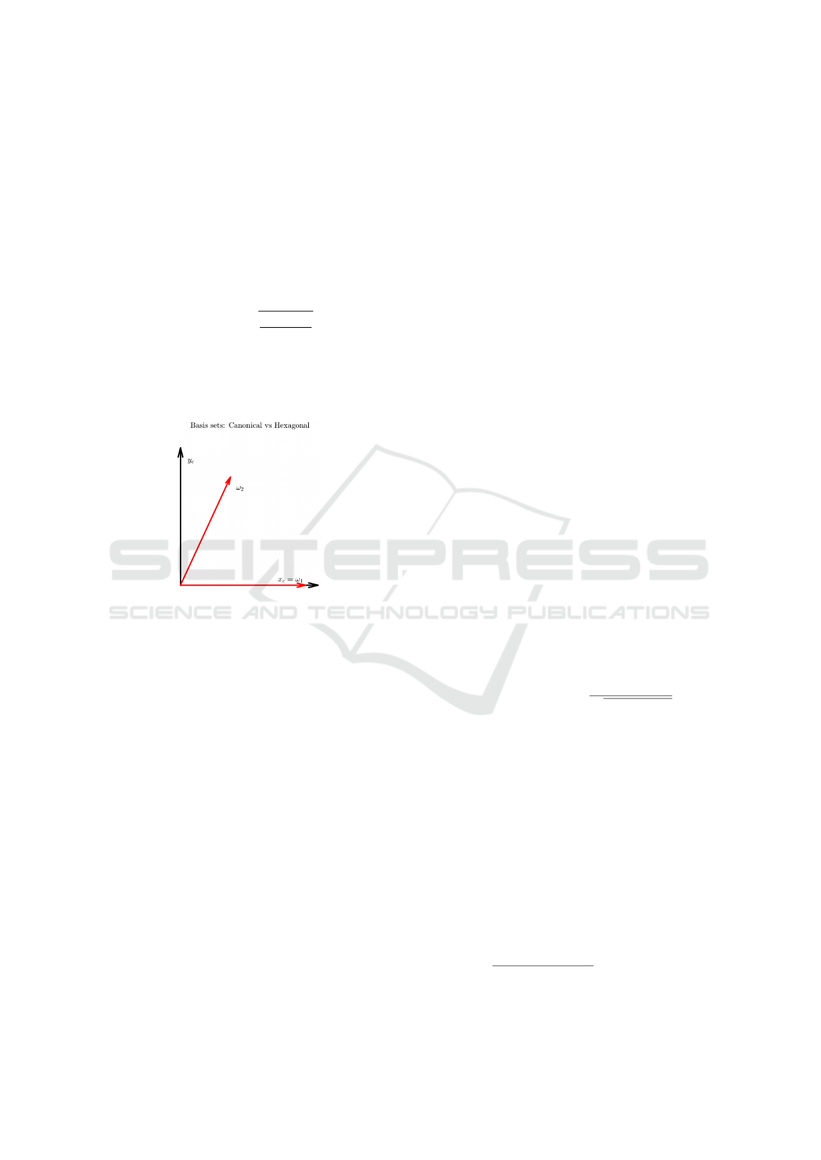
These basis vectors are shown in red colour in Fig-

ure 1 in R

, while the canonical vectors are shown in

black.

Figure 1: Black: Canonical basis. Red: Hexagonal basis

set.

Although any scattered points could be used as

collocation points, the hexagonal grid has been shown

to minimize the condition numbers of the collocation

matrices for a ﬁxed ﬁll distance, i.e. a measure of the

density of the collocation grid (Iske, 1998).

Since f(x) = 0 for all equilibria x, we remove all

equilibria from the set of collocation points X; not do-

ing so would cause the collocation matrix to be singu-

lar.

The ﬁrst approximation v to a complete Lyapunov

function is then given by the function that satisﬁes

the PDE v

(x) = −1 at all collocation points and is

norm minimal in the corresponding Reproducing Ker-

nel Hilbert space H.

In later iterations we solve v

(x) = r

for different

≤ 0, determined by previous approximations.

Practically, we compute v by solving a system of

N linear equations, where N is the number of colloca-

tion points.

The explicit formulas for v and its orbital deriva-

tive are

v(x) =

∑

j=1

−x, f(x

)iψ

(kx −x

k),

(x) =

∑

j=1

−ψ

(kx −x

k)hf(x),f(x

+ψ

(kx −x

k)hx −x

,f(x)i

·hx

−x, f(x

where ψ

,ψ

are functions computed from the Wend-

land function ψ

l,k

used, h·,·i denotes the standard

scalar product and k· k the Euclidean norm in R

β ∈ R

is the solution to Aβ = r, r

= r(x

) and A

is the N ×N matrix with entries

i j

= ψ

(kx

−x

k)hx

−x

,f(x

)ihx

−x

,f(x

)i (4)

−ψ

(kx

−x

k)hf(x

),f(x

for i 6= j and

= −ψ

(0)kf(x

More detailed explanations on this construction are

given in (Giesl, 2007, Chapter 3).

If no collocation point x

is an equilibrium for the

system, i.e. f(x

) 6= 0 for all j, then the matrix A is

positive deﬁnite and the system of equations Aβ = r

has a unique solution.

The last assertion will hold true independently of

whether the underlying discretized PDE has a solu-

tion or not, while error estimates are obviously only

available if the PDE has a solution.

Note that in the context of RBF, a positive deﬁnite

function ψ refers to the matrix (ψ(kx

−x

k))

i, j

being

positive deﬁnite for X = {x

,.. . ,x

}, where x

if i 6= j.

As explained in (1), in (Arg

aez et al., 2018b) we

introduced an “almost” normalized approach, i.e., the

original dynamical system (1) was substituted by

x =

f(x), where

f(x) =

f(x)

+ kf(x)k

(5)

with a small parameter δ > 0. This normalization al-

ready reduces signiﬁcantly the overestimation of the

chain-recurrent set.

2.4 Evaluation Grid

After we have solved the PDE numerically, i.e. forced

) = −r

at every collocation point x

, we use an

evaluation grid Y

around each collocation point x

to evaluate the results.

Placing all evaluation points aligned to the ﬂow

of the ODE system, as introduced in (Arg

aez et al.,

2018c; Arg

aez et al., 2018a), has proved successful.

The formula for the evaluation grid is

(

r ·k ·α

Hexa-basis

f(x

)

f(x

: k ∈ {1, .. ., m}

)

SIMULTECH 2019 - 9th International Conference on Simulation and Modeling Methodologies, Technologies and Applications

144

where α

Hexa-basis

is the parameter used to build the

hexagonal grid deﬁned above, r ∈ (0,1) is the ratio

up to which the evaluation points will be placed and

m ∈N denotes the number of points in the evaluation

grid that will be placed on both sides of the colloca-

tion points aligned to the ﬂow.

Using this evaluation grid means that there will

not be any evaluated points to provide information

about the dynamical system other than in the direction

of the ﬂow. However, this evaluation grid avoids ex-

ponential growth of evaluation points as the system’s

dimension becomes higher and the results are usually

good, i.e. enough information about the dynamics is

gained.

We start by computing the approximate solution

to V

(x) = −1 with collocation points X. As we

have previously done in (Arg

aez et al., 2017; Arg

aez

et al., 2018b), we deﬁne a tolerance parameter −1 <

γ ≤ 0. In each step i of the iteration we mark a col-

location point x

as being in the chain-recurrent set

∈ X

) if there is at least one point y ∈ Y

such

that v

(y) > γ. The points for which the condition

(y) ≤ γ holds for all y ∈ Y

are considered to be-

long to the gradient-like ﬂow (x

∈ X

−

As has been done in (Arg

aez et al., 2018c), in this

paper we replace the right-hand side −1 by the aver-

age of the values v

(y) over the evaluation grid y ∈Y

at each collocation point x

for averages that are neg-

ative. In cases in which the average is positive we use

0. In formulas, we calculate the approximate solution

i+1

of V

) = ˜r

with

˜r





∑

y∈Y

(y)





−

where x

−

= min(0,x). We will refer to this as the

“non-scaled” version.

However, this approach can lead to a continuous

decrease of “energy” over the iterations.

Recall that the original value of the orbital deriva-

tive condition in the ﬁrst iteration is −1, but the new

value is obtained by averaging and bounding by 0.

This can cause it to converge to zero and thus force the

total “energy” of the Lyapunov function to decrease.

To avoid this, we scale the condition of the orbital

derivative after the ﬁrst iteration onwards so that the

sum of all r

over all collocation points is constant

for all iterations; we will refer to this as the “scaled”

method.

Our algorithm to compute complete Lyapunov

functions and classify the chain-recurrent set can be

summarized as follows:

1. Create the set of collocation points X and compute

the approximate solution v

to V

(x) = −1; set i = 0

2. For each collocation point x

, compute v

(y) for

all y ∈ Y

: if v

(y) > γ for a point y ∈ Y

, then

∈X

, otherwise x

∈X

−

, where γ ≤ 0 is a cho-

sen critical value

3. Deﬁne ˜r



∑

y∈Y

(y)



−

4. Deﬁne r

∑

l=1

|˜r

˜r

5. Compute the approximate solution v

i+1

) = r

for j = 1, . ..,N; this is the scaled

version, while approximating the solution of

) = ˜r

would be the non-scaled version

6. Set i → i + 1 and repeat steps 2. to 5. until no

more points are added to X

Note that the sets X

and X

−

may change at each step

of the algorithm.

3 MIDDLE POINT REDUCTION

3.1 Middle Point Algorithm

Once we have obtained our approximations X

and

−

to the chain-recurrent and gradient-like ﬂow re-

spectively, we want to classify the points X

in the

chain-recurrent set into its different connected com-

ponents, e.g. different orbits and equilibria.

The way of doing it follows the algorithm ex-

plained in (Arg

aez et al., 2019a).

A brief description is given below:

Algorithm 3.1: Once the chain-recurrent set is obtained.

1. Measure all distances from the origin to the dif-

ferent failing points

2. Sort all points in an increasing order according to

their distance from the origin

3. Measure the difference in radii-length between

every two consecutive points. Gaps are consid-

ered to happen when difference in distance is

greater than α

Hexa-basis

for two consecutive points

4. All points before the ﬁrst gap are considered to

be a part of the ﬁrst set of connected components.

Between the ﬁrst and the second gap, all points

are considered to be part of the second set of con-

nected component, etc. After we have found all

gaps, the last one of them and the longest radius

length deﬁne the last set of connected components

5. Each set of component is decomposed into its

connected components

Middle Point Reduction of the Chain-recurrent Set

145

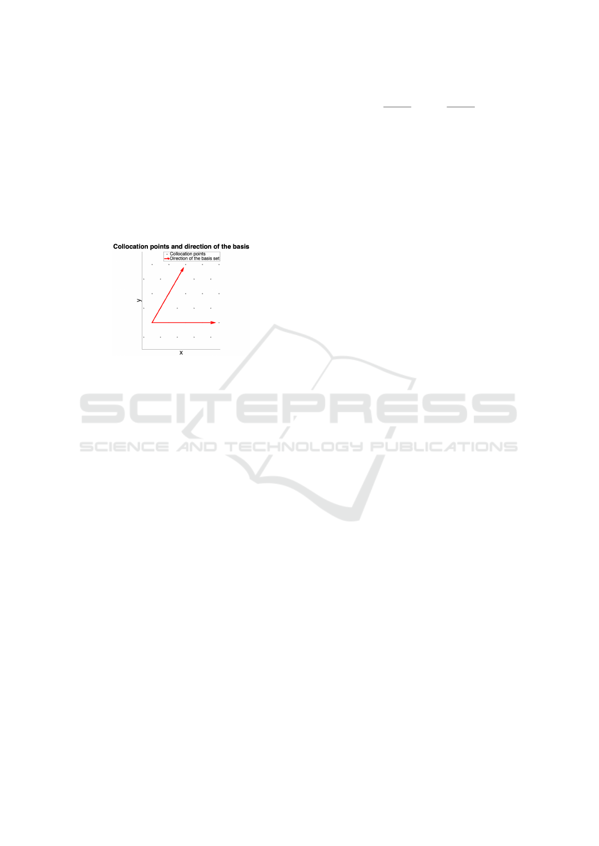
Let us point out that the chain-recurrent set is

given by the points in the collocation grid that failed

the approximation.

Therefore, they will all be aligned to the basis set

of vectors of the hexagonal grid, see Figure 2.

For each point in this classiﬁcation of the chain-

recurrent set, we will build two groups. One will con-

sist of all its neighbours and neighbours of its neigh-

bours, etc., aligned to the ﬁrst basis vector. The sec-

ond will consist of all its neighbours and neighbours

of its neighbours, etc., aligned to the second basis vec-

tor.

Figure 2: Points in the collocation grid aligned to the hexag-

onal basis set. Distance between two consecutive points is

Hexa−basis

Given a point x

in a sub-classiﬁcation of the

chain-recurrent set, a way of obtaining the most di-

rect neighbours in a direction of a vector ω

in the

hexagonal basis (3) is to “walk” positively and neg-

atively in the sense of that direction, with steps of

size α

Hexa−basis

. That is, consider the points x

jα

Hexa−basis

for integer j. Then, the neighbours of

its neighbours will be found with the “next step”, etc.

When a next pth-step is given and no point is found,

then the search in that direction’s sense is stopped.

The total search of neighbours for that point stops

when both direction’s senses, the positive and the

negative, reach a point that was not originally in the

chain-recurrent set. Then, the new sub-classiﬁcation

group continues with another point.

Once we have grouped all the points in the sub-

classiﬁcation of chain-recurrent set, then each indi-

vidual group is organized by its different distances be-

tween points. The two most far-apart points in each

group are the boundaries of that group in that direc-

tion. These two points give, in that particular direc-

tion, the middle point that we are looking for to obtain

the reduction.

We consider that the reduced chain-recurrent set

is the total union of the middle points for each point’s

group in both directions.

Let us recall that the middle point of two points

) and (x

) is given by,

+ x

, y

+ y

(6)

Single points in the orbit will be themselves after

the reduction as they are, themselves, their middle-

points. For one dimensional chain-recurrent set, the

algorithm is listed bellow.

Begin

1) Construct the Lyapunov function and its orbital

derivative;

2) Obtain the chain-recurrent set;

3) Divide it into its connected components

4) For each point in the chain-recurrent set build a

group of adjacent collocation points in direction ω

and one in direction ω

5) Identify groups that are equal 6) Find the extreme

points in each group and replace the points in the

group by the middle point

7) The reduced chain-recurrent set is the collection of

all middle points

8) Merge all groups aligned with ω

into a another set

of groups

9) For each group apply the middle points formula 10)

The reduced chain-recurrent set is the collection of all

middle points

End.

4 RESULTS

4.1 Two Periodic Orbits

We consider system (1) with right-hand side

f(x,y) =



−x(x

+ y

−1/4)(x

+ y

−1) −y

−y(x

+ y

−1/4)(x

+ y

−1) + x



(7)

This system has an asymptotically stable equilibrium

at the origin. Moreover, the system has two periodic

circular orbits: an asymptotically stable periodic orbit

at Ω

= {(x,y) ∈ R

| x

+ y

= 1} and a repelling

periodic orbit at Ω

= {(x, y) ∈ R

| x

+ y

= 1/4}.

To compute the complete Lyapunov function with

our method we used the Wendland function ψ

5,3

. The

collocation points were set in a region [−1.5,1.5] ×

[−1.5,1.5] ⊂ R

and we used a hexagonal grid (3)

with α

Hexa−basis

= 0.0162. The evaluation grid was

computed with the directional grid (6) with parameter

m = 50.

We computed this example with the almost-

normalized method

x =

f(x) with δ

= 10

−8

and γ =

−0.8.

Figure 4 shows the complete Lyapunov function

and its orbital derivative computed using 3 iterations.

The two orbits with radii 1/2 and 1 can clearly be

SIMULTECH 2019 - 9th International Conference on Simulation and Modeling Methodologies, Technologies and Applications

146

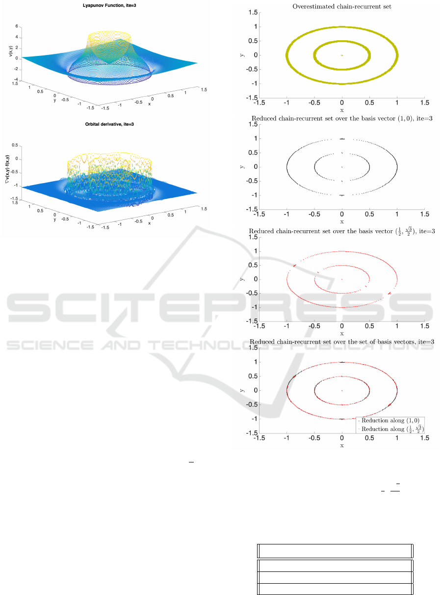
Figure 3: Upper: Complete Lyapunov function for system

7. Lower: Orbital derivative for system 7.

identiﬁed. The ﬁrst one is a repeller and the second is

attractive. We see that beyond the second orbit with

radius 1, the behaviour of the Lyapunov function is

well behaved and its orbital derivative whose value

approximated −1 nicely. However, at the orbits and

close to the equilibrium at zero, we can see that the

orbital derivative fails the approximation. The collo-

cation points associated to the failing point are shown

in the last ﬁgure of Figure 3 in dark-yellow colour.

That is our approximation to the chain-recurrent set.

The middle-point reduced the chain-recurrent set over

the vector basis (1,0) is shown in the upper ﬁgure of

3. The two dots representing the equilibrium point at

the origin, the middle point reduction, are the same as

the original ones before reduction. They did not have

neighbours within a α

Hexa−basis

distance. As such,

the middle-up ﬁgure shows the middle-point reduced

chain-recurrent set over the vector basis (1/2,

√

3/2),

Figure 3. It is interesting to notice that in different

directions there will be different areas without points.

It is the union of both groups, lowest ﬁgure in Figure

3, that gives the total reduction.

The ﬁnal reduction is shown over the ﬁrst over-

estimated chain-recurrent set at the bottom of Figure

3. Let us show in numbers what the reduction means,

Table 1.

Table (1) shows the number of elements in the

chain-recurrent set in both cases: The non-reduced

and the reduced one. As can be seen, the number

of elements after the reduction can be a half of the

amount of numbers before the reduction.

Figure 4: Upper: Overestimated chain-recurrent set with

γ = 0.8. Middle up: Middle point reduction over the hexag-

onal basis vector (1, 0). Middle down: Middle point re-

duction over the hexagonal basis vector



√



. Bottom:

Both reductions. All ﬁgures for system (7).

Table 1: Difference in the total amount of points per section

of the chain-recurrent set for example (7).

Section Before After

Equilibrium point 2 2

Orbit r = 1/2 612 256

Orbit r = 1 1062 512

Middle Point Reduction of the Chain-recurrent Set

147

4.2 Van der Pol Oscillator



˙x

˙y



= f(x, y) =



(1 −x

)y −x



. (8)

For computing the complete Lyapunov function as-

sociated to system (8), we set α

Hexa-basis

= 0.043 over

the area deﬁned by [−4,4]

⊂ R

. The Wendland

function parameters used are (l, k,c) = (4,2,1), the

critical value γ = −0.5, and δ

= 10

−8

. The evalua-

tion grid was computed with the directional grid with

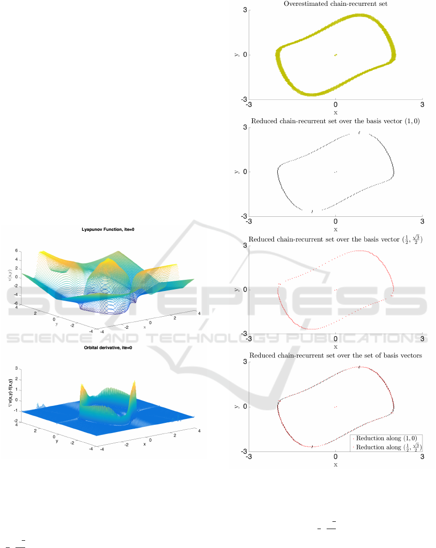
m = 10. The complete Lyapunov function at the ini-

tial iteration and the orbital derivative over the chain-

recurrent set is shown in Figure 5.

As can be seen, the Lyapunov function has a re-

peller at the origin and it has a non-circular but still

symmetric orbit around the origin. Away from the

orbit, the orbital derivative satisﬁes the condition −1

nicely but again the approximation fails in the orbit,

the repeller and the points nearby.

Figure 5: Upper: Complete Lyapunov function for system

8. Lower: Orbital derivative for system (8).

Our approximated chain-recurrent set is shown

in the last ﬁgure of Figure 5 in dark-yellow colour.

Again the upper ﬁgure shows the reduction along

(1,0) and middle-upper ﬁgures the reduction along

(

√

). The total middle-point reduction is again

shown in ﬁgure middle-lower of Figure 6. The re-

duction becomes clear when seen over the original

estimation of the chain-recurrent set, lower ﬁgure in

Figure 6.

Figure 6: This ﬁgure shows both the overestimation and

the reductions. It is divided in four subﬁgures. Upper:

Overestimated chain-recurrent set with γ = 0.043. Middle

up: Middle point reduction over the hexagonal basis vec-

tor (1,0). Middle down: Middle point reduction over the

hexagonal basis vector



√



Bottom: Both reductions.

All ﬁgures for system (8).

In Table 2 the reduction is quantiﬁed. The table shows

that the number of elements is reduced to circa a third

of its original overestimated value.

SIMULTECH 2019 - 9th International Conference on Simulation and Modeling Methodologies, Technologies and Applications

148

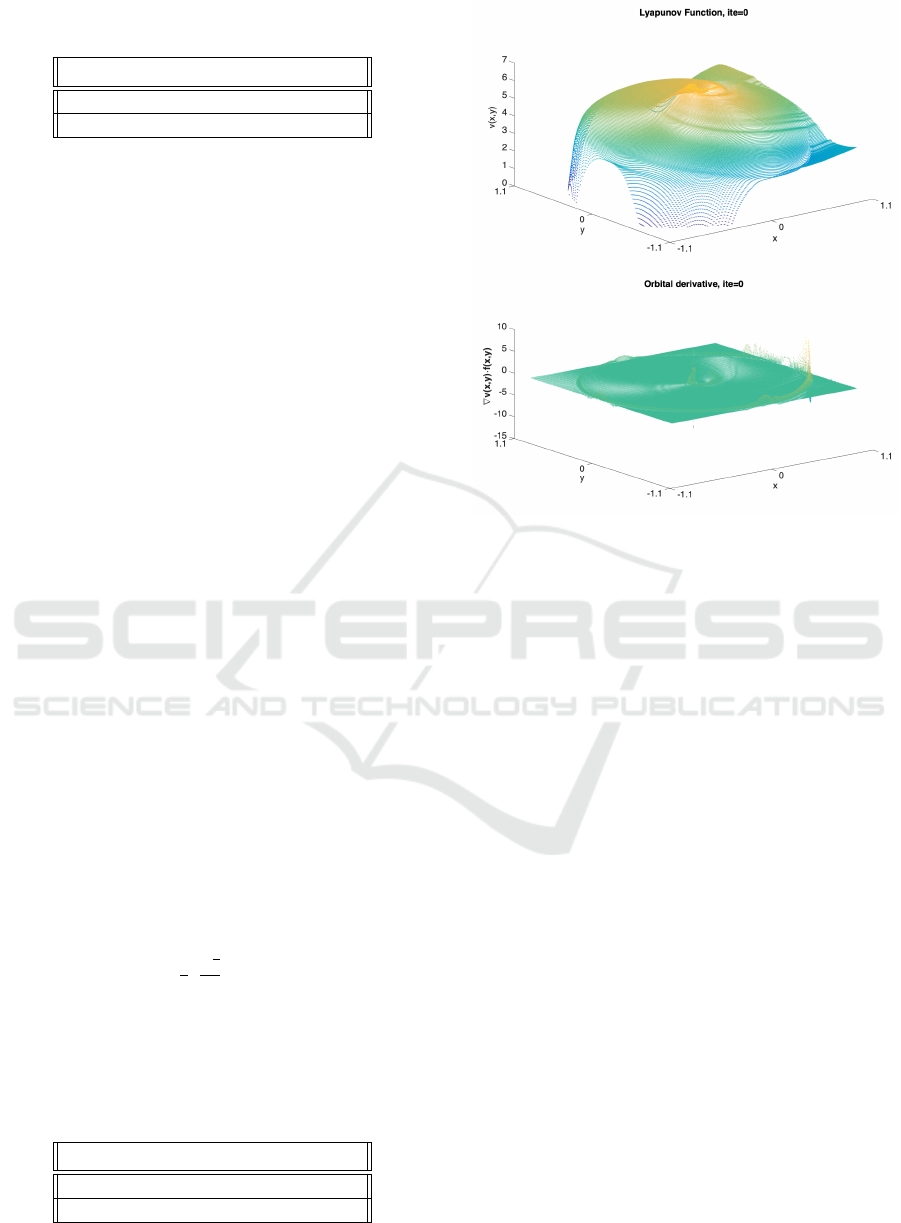
Table 2: Difference in the total amount of points per section

of the chain-recurrent set for example (8).

Section Before After

Equilibrium point 2 2

Limiting orbit 1212 444

4.3 Homoclinic Orbit

As in (Arg

aez et al., 2017), we also consider here the

following example



˙x

˙y



= f(x, y) (9)



x(1 −x

−y

) −y((x −1)

+ (x

+ y

−1)

)

y(1 −x

−y

) + x((x −1)

+ (x

+ y

−1)

)



The origin is an unstable focus and the system has

an asymptotically stable homoclinic orbit at a cir-

cle centred at the origin and with radius 1, con-

necting the equilibrium (1,0) with itself. We used

the Wendland function ψ

4,2

for our computations.

Our collocation points were deﬁned in the region

[−1.1,1.1] ×[−1.1, 1.1] ⊂ R

with a hexagonal grid

(3) with α

Hexa−basis

= 0.011. In this example, we have

used the normalized method, i.e. we replaced f by

f as

in (5) with δ

= 10

−8

, and we used γ = −0.75. As

before, the evaluation grid was computed with the di-

rectional grid with m = 10. The complete Lyapunov

function and its orbital derivative are shown in Figure

The Lyapunov function has a maximum at the ori-

gin which is a repelling equilibrium point. The orbit

can be seen at radius 1. The orbital derivative condi-

tion approximates very well the condition −1 every-

where except in the orbit and in the origin. The ap-

proximated chain-recurrent set is shown at the lower

ﬁgure of Figure 7 in dark-yellow colour. Figure 8 has

four subﬁgures. The upper ﬁgure shows the overes-

timation. The middle-upper one is the middle-point

reduction over (1,0). The middle-lower is the middle-

point reduction over



√



. The lowest is the union

of both.

Let us show in numbers what the reduction means,

table 3.

Table 3: Difference in the total amount of points per section

of the chain-recurrent set for problem 9.

Section Before After

Equilibrium point 255 86

Homoclinic orbit 1579 941

Figure 7: Upper: Complete Lyapunov function for system

9. Lower: Orbital derivative for system 9. This ﬁgures

where obtain after just one iteration.

5 DISCUSSION

Let us discuss the results by analysing ﬁrst the ho-

moclinic orbit example. The orbit has a circumfer-

ence of radius r = 1. The α

Hexa-basis

parameter for

that problem was set to be α

Hexa-basis

= 0.011. That

would let us assume that the total amount of colloca-

tion points that should be given in the orbit is the total

perimeter divided by α

Hexa-basis

, that is: P/α

Hexa-basis

2πr/0.011 = 571 points. In that calculation P rep-

resents the perimeter of the orbit. The ﬁrst overes-

timated approximation we obtained had 1579 on the

orbit with radius r = 1, so it was 276% overestimated.

The middle point reduction gave 165% overestima-

tion. So, 111% less.

One could think that these new results happen to

be overestimated as well. However, this is not the

case. They are in fact good results because the middle

point reduction is placing points over the orbit where

collocation points where not even deﬁned. That is,

between two different collocation points. Figure 9

shows this in a pedagogical way:

Figure 9 shows middle-point reductions in be-

tween different collocation points. So, the distance

between two consecutive points in the reduction is

now, α

Hexa-basis

/2 = 0.0055. In the ideal case in which

all points were placed equidistantly that would make

Middle Point Reduction of the Chain-recurrent Set

149

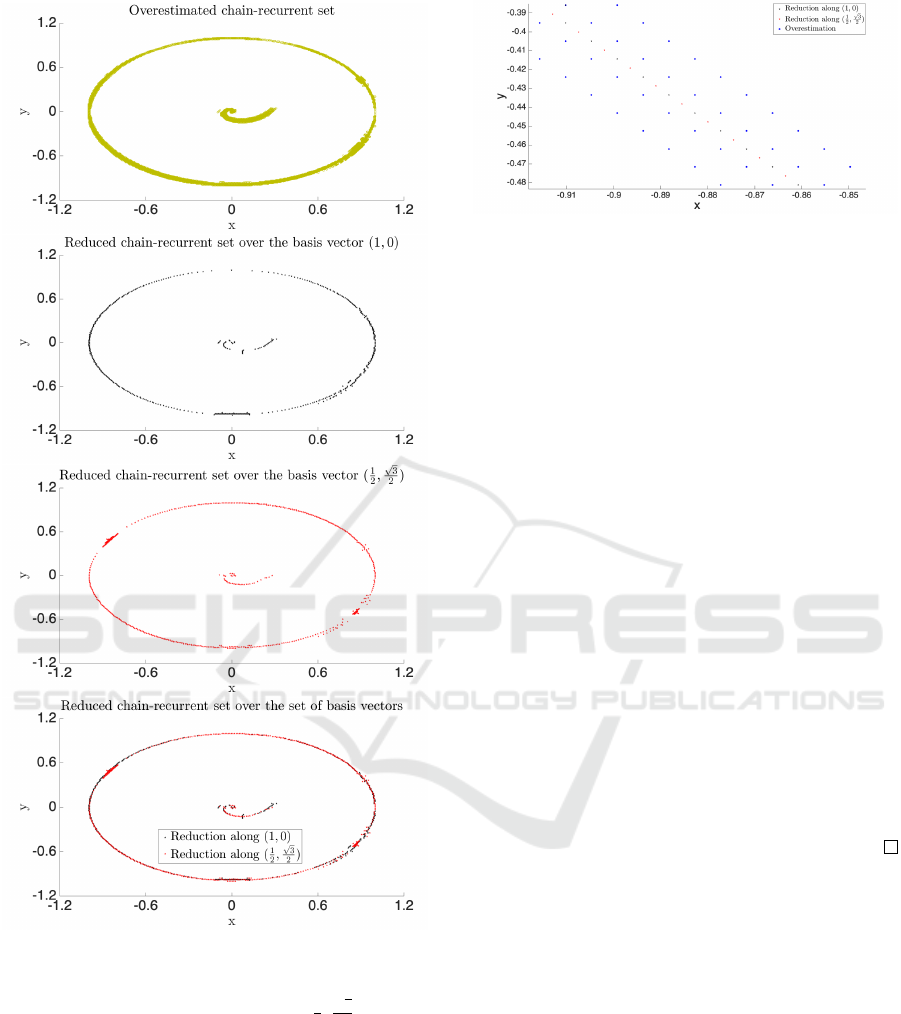
Figure 8: Upper: Overestimated chain-recurrent set with

γ = −0.75. Middle up: Middle point reduction over the

hexagonal basis vector (1,0). Middle down: Middle point

reduction over the hexagonal basis vector



√



Bottom:

Both reductions. All ﬁgures for example (9).

a total number of P/α

Hexa-basis

= 2πr/0.0055 = 1142

points. However, not all points in the middle point

reduction are placed equidistantly.

Now, the equilibrium point is overestimated with

86 points. That is because the chain-recurrent set

approximation failed from the beginning with 255

points. That makes a reduction of over 70%.

Similar analysis can be made for examples (7) and

Figure 9: Middle point reductions seen around the colloca-

tion points.

(8). However, in these last cases, the equilibrium

point is better estimated.

These results lead us to enunciate the following

lemma.

Lemma 5.1 (Middle point reduction). Under the

middle-point reduction to a closed orbit of a Lya-

punov function constructed with the algorithm de-

scribed in Sec. 2. The cardinality of elements in the

reduction will be bounded below by P

/α

Hexa-basis

Where P

> 1 is the perimeter of the closed orbit

and α

Hexa-basis

< 1 is the parameter to build collocation

grid.

Proof. Given the geometric conditions used to build

the collocation points, the reduced points can be as

much as α

Hexa-basis

apart. That will only happen if all

the middle points reductions give a point that already

belong to the collocation grid. If on the other hand,

the middle point reduction gives only new points, then

by construction the new points will be placed between

elements of the collocation grid and again, they will

be apart by α

Hexa-basis

Therefore, the total amount of points in the reduc-

tion will be always bounded below by P

/α

Hexa-basis

6 OBSERVATIONS

In (Arg

aez et al., 2019c), we made a large analysis of

the cost of computing an approximation to a complete

Lyapunov function with our method using I iterations.

That analysis is carried out under the big-oh approach.

It was proven that our computation is as expen-

sive as O(N

+ IN

nm) where N is the total number

of collocation points, n is the dimension of the prob-

lem and m the total amount of points to be evaluated

in the evaluation grid.

Generating the different groups aligned to the dif-

ferent vector basis set is built with two for-loops per

orbit. However, the total amount of failing points, µ,

i.e. points in the chain-recurrent set, is much lower

SIMULTECH 2019 - 9th International Conference on Simulation and Modeling Methodologies, Technologies and Applications

150

than N. So, a for-loop is carried to all points in the

chain-recurrent set, per each point, p steps are given

in both directions of the basis set. Finally, each new

point is checked to belong to the chain-recurrent set.

So, the total cost is µ

p with p < µ < N. Therefore,

the total cost of constructing the complete Lyapunov

function remains O(N

+ IN

nm).

It is to be pointed out that the example 8 is actually

an example arising from engineering. It represents the

limiting cycles in electrical circuits built with vacuum

tubes. Therefore this is a real-life application of our

methodology.

7 CONCLUSIONS

We have introduced an algorithm capable of reduc-

ing the overestimation of the chain-recurrent set. This

algorithm is based on exploring the geometrical con-

straints used to construct the complete Lyapunov

function in the ﬁrst place. Grouping the elements of

the chain-recurrent subsets (or orbits) into different

small groups of points aligned to the hexagonal basis

vectors allowed us to obtain the corresponding middle

points. The new points obtained over the orbit can be

added to the collocation points for further iterations

and constraints. However, that will be done in future

work.

An important observation to be made is that al-

though the elements of the different groups are always

elements of the hexagonal collocation grid, the mid-

dle points might not be part of it. However, it was

to be expected that the continuous orbit would pass

through the spaces between two consecutive colloca-

tion points. That enlightens the fact that the denser

the collocation points grid is, the better the results.

Furthermore, since we know that these points have

zero orbital derivative, one could now re-build the

complete Lyapunov function with the right condition

on that particular set without forcing extra points to be

zero; optimizing our new approximation to the com-

plete Lyapunov function.

However, a remaining problem to solve is an

equivalent algorithm capable to work in higher di-

mensions.

Finally, our method has been applied to a real-

world application problem arising from electrical en-

gineering, as our results for equation (8) shows.

ACKNOWLEDGEMENTS

The ﬁrst author in this paper is supported by the Ice-

landic Research Fund (Rann

ıs) grant number 163074-

052, Complete Lyapunov functions: Efﬁcient numer-

ical computation.

REFERENCES

Arg

aez, C., Giesl, P., and Hafstein, S. (2017). Analysing

dynamical systems towards computing complete Lya-

punov functions. In Proceedings of the 7th In-

ternational Conference on Simulation and Modeling

Methodologies, Technologies and Applications (SI-

MULTECH), pages 134–144. Madrid, Spain.

Arg

aez, C., Giesl, P., and Hafstein, S. (2018a). Computation

of complete Lyapunov functions for three-dimensional

systems. In Proceedings IEEE Conference on Deci-

sion and Control (CDC), 2018, pages 4059–4064. Mi-

ami Beach, FL, USA.

Arg

aez, C., Giesl, P., and Hafstein, S. (2018b). Compu-

tational approach for complete Lyapunov functions.

In Dynamical Systems in Theoretical Perspective.

Springer Proceedings in Mathematics & Statistics. ed.

Awrejcewicz J. (eds)., volume 248.

Arg

aez, C., Giesl, P., and Hafstein, S. (2018c). Iterative

construction of complete Lyapunov functions. In Pro-

ceedings of the 8th International Conference on Sim-

ulation and Modeling Methodologies, Technologies

and Applications (SIMULTECH). Porto, Portugal.

Arg

aez, C., Giesl, P., and Hafstein, S. (2019a). Clustering

algorithm for generalized recurrences using complete

Lyapunov functions. In International Conference on

Informatics in Control, ICINCO. SUBMITTED.

Arg

aez, C., Giesl, P., and Hafstein, S. (2019b). Improved

estimation of the chain-recurrent set. In ECC 2019,

Naples.

Arg

aez, C., Giesl, P., and Hafstein, S. (2019c). Iterative

construction of complete lyapunov functions: Analysis

of algorithm efﬁciency. In Springer. SUBMITTED.

Bernhard, P. and Suhr, S. (2018). Lyapounov functions of

closed cone ﬁelds: From Conley theory to time func-

tions. Commun. Math. Phys., 359:467–498.

Conley, C. (1978). Isolated Invariant Sets and the Morse In-

dex. CBMS Regional Conference Series no. 38. Amer-

ican Mathematical Society.

Conley, C. (1988). The gradient structure of a ﬂow I. Er-

godic Theory Dynam. Systems, 8:11–26.

Dellnitz, M. and Junge, O. (2002). Set oriented numeri-

cal methods for dynamical systems. In Handbook of

dynamical systems, Vol. 2, pages 221–264. North-

Holland, Amsterdam.

Fathi, A. and Pageault, P. (2019). Smoothing Lyapunov

functions. Trans. Amer. Math. Soc., 371:1677–1700.

Giesl, P. (2007). Construction of Global Lyapunov Func-

tions Using Radial Basis Functions. Lecture Notes in

Math. 1904, Springer.

Giesl, P., Arg

aez, C., Hafstein, S., and Wendland, H. (2018).

Construction of a complete Lyapunov function using

quadratic programming. In Proceedings of the 15th

International Conference on Informatics in Control,

Automation and Robotics (ICINCO). SIMULTECH

2018, Porto.

Middle Point Reduction of the Chain-recurrent Set

151

Hsu, C. S. (1987). Cell-to-cell mapping, volume 64 of Ap-

plied Mathematical Sciences. Springer-Verlag, New

York.

Hurley, M. (1995). Chain recurrence, semiﬂows, and gra-

dients. J Dyn Diff Equat, 7(3):437–456.

Hurley, M. (1998). Lyapunov functions and attractors in

arbitrary metric spaces. Proc. Amer. Math. Soc.,

126:245–256.

Iske, A. (1998). Perfect centre placement for radial basis

function methods. Technical Report TUM-M9809, TU

Munich, Germany.

Krauskopf, B., Osinga, H., Doedel, E. J., Henderson, M.,

Guckenheimer, J., Vladimirsky, A., Dellnitz, M., and

Junge, O. (2005). A survey of methods for computing

(un)stable manifolds of vector ﬁelds. Internat. J. Bifur.

Chaos Appl. Sci. Engrg., 15(3):763–791.

Lyapunov, A. M. (1992). The general problem of the sta-

bility of motion. Internat. J. Control, 55(3):521–790.

Translated by A. T. Fuller from

Edouard Davaux’s

French translation (1907) of the 1892 Russian orig-

inal.

Wendland, H. (1998). Error estimates for interpolation by

compactly supported Radial Basis Functions of mini-

mal degree. J. Approx. Theory, 93:258–272.

SIMULTECH 2019 - 9th International Conference on Simulation and Modeling Methodologies, Technologies and Applications

152