
Kinematics Modelling, Optimization and Control
of Hybrid Robots
Mahmoud Tarokh
a
and Federico Llenar
Department of computer Science, San Diego State University, San Diego, CA 92182-7720, U.S.A.
Keywords: Hybrid Robots, Rolling and Walking Kinematics.
Abstract: The paper develops a unified kinematics modelling, optimization and control for hybrid robots. These
robots combine two or more modes of operations, such as a combination of walking and rolling, or rolling
and manipulation. The equations of motion are derived in compact forms that embed an optimization
criterion. These equations are used to obtain various useful forms of the robot kinematics. Using the
developed modelling, actuation and control equations are derived that ensure the robot to track a desired
path closely while maintaining balanced operations and tip-over avoidance. Various simulation results are
provided for a hybrid rolling-walking robot traversing uneven terrain, which demonstrate the capabilities
and effectiveness of the developed methodologies.
1 INTRODUCTION
Robots are becoming more sophisticated in
mechanisms, control and intelligence to enable
execution of complex tasks in challenging
environments. In order to perform such tasks,
various hybrid robots capable of multiple modes of
operations such as combinations of rolling and
walking, and rolling and manipulation as in mobile
manipulators, have been proposed. In particular,
hybrid locomotion of walking and rolling has
received special attention. This is due to the fact that
walking robots have superior performance for
traversing uneven terrain. On the other hand rolling
robots are better suited for relatively flat terrains as
they can move faster and are more stable than
walking robots in such terrain.
There are various methods to combine
propulsion. Most mecha
a
nisms mount wheels at the
end of legs that can be locked to act as feet. Robots
that have been developed based on this mechanical
architecture are usually four legged wheel-foot
arrangements. These include Hylos (Grand et al,
2000), Paw (Smith et al, 2006), Primres-Sherpa
(Cordes et al, 2011) and Workpartner (Ylonen and
a
https://orcid.org/0000-0002-1846-4570
Halme, 2002). The use of more than four legs adds
to the complexity but also offers more versatility and
extends application and behavioural diversity, such
as stair climbing (Yuan and Hirose, 2004), high load
carrying capability (Fujita and Sasaki, 2017),
learning new locomotion when a leg is damaged
(Cully et al, 2015; Jehanno et al 2014) and a highly
articulated legged wheel-foot robot (Siegwart et al,
2002).
Kinematics analysis and motion control of wheeled
robots and legged-foot robots have followed very
different methodologies. The kinematic modelling of
ordinary wheeled robots moving on flat surfaces was
developed in (Muir and Neuman, 1991), and
extended in (Rajagopalan, 1997), (Shin et al, 2001).
The kinematics modelling of articulated rovers
traversing uneven terrain poses a number of
challenging problems that are much more
complicated than the ordinary mobile robots moving
over flat terrain. The first research work on
kinematics modelling of an articulated wheeled
robot over uneven terrain appears to be given in
(Tarokh et al, 1999). In this work the kinematics of
the Rocky 7 Mars rover is formulated. This work
was subsequently generalized allowing modelling
and analysis of rovers with active suspension
systems (Tarokh and McDermott 2005), (Tarokh and
McDermott, 2007) where three types of kinematics,
namely navigation, actuation and slip kinematics,
were identified and motion control was suggested.
114
Tarokh, M. and Llenar, F.
Kinematics Modelling, Optimization and Control of Hybrid Robots.
DOI: 10.5220/0007915801140123
In Proceedings of the 16th International Conference on Informatics in Control, Automation and Robotics (ICINCO 2019), pages 114-123
ISBN: 978-989-758-380-3
Copyright
c
2019 by SCITEPRESS – Science and Technology Publications, Lda. All rights reserved

Subsequently, balance control and a
recursiveformulation of the kinematics for general
articulated rovers were developed in (Tarokh et al,
2006), (Tarokh and Ho, 2013). More recently, (Kelly
and Seegmiller, 2015) proposed a recursive
formulation based on a differential algebraic
formulation of the robot kinematics (Kelly, 2012)
There has been extensive work on motion
planning of legged walking robots ranging from the
mechanical considerations to foot placement,
stability and gait optimization. A main consideration
in walking robots is the stability and tip-over
avoidance. Various techniques have been proposed,
many based on the so called zero-moment-point
(ZMP) and its modification (Winkler et al, 2017).
An inverse kinematics is developed in (Shkolnik and
Tedrake, 2007) for controlling the center of mass
and the swing leg trajectory. A motion control of
walking is proposed in (Zhong, 2016) using
decentralized controller for a hexapod walking
robot. Furthermore, (Winkler et al, 2018) proposes a
trajectory optimization to determine gait sequence,
foothold and swing leg motion. In order to achieve
various dynamic gaits such as pace, trot and jumping
(Bellicoseo et al, 2018) develops dynamic
locomotion through nonlinear motion optimization.
The above mentioned papers and others propose
variety of different methods for kinematics analysis
and control, each applicable to a particular type of
robot, i.e. rovers, walking robots, and mobile
manipulators. However, there does not appear to
exist a unified kinematics modelling and
performance optimization that can be equally
applied to hybrid robots with multiple modes of
operations. In this paper we develop a unified
kinematics modelling and control, incorporating
optimization, for hybrid robots. Section 2
characterizes hybrid robots and various components
needed for analysis, optimization and control.
Section 3 develops kinematics modelling for hybrid
robots. Optimization and control are discussed in
Section 4. Simulation results for two modes of
operation of a hybrid robot are provided in Section
5. Finally, Section 6 outlines the conclusions of the
work.
2 CHARACTERIZATION OF
GENERAL HYBRID ROBOTS
We define a general hybrid robot as the one with a
body that is connected to a set of limbs, i.e. arms and
legs. Each limb consists of a number of links and
joints which can be prismatic, revolute, or a
combination of these. An arm is attached to a base
and is terminated at an end-effector (hand) which is
generally free to move in its workspace and can
manipulate objects. On the other hand, a leg-end
(wheel, foot, etc.) is generally in contact with the
environment. A leg can be terminated at any one of
the following: (i) a wheel for rolling on the terrain as
in rovers and mobile robots, (ii) a foot that can be
held on the terrain or lifted up and move as in
walking robots, (iii) a wheel with a mechanism that
can be locked so that it can act as a foot for walking
or unlocked for rolling. This is the case for hybrid
rolling and walking robots, (iv) a leg with simple or
compound joints that connects a fixed base to a top
platform and adjusts the position and orientation of
the top platform by changing the leg length as in
Stewart-type platforms.
A leg-end can be constrained, e.g. wheels of a
rover or stance leg of a walking robot that are in
contact with the terrain. It can also be free to move
such as a swing leg of a walking robot.
A joint can be active (actuated) for adjusting its
value, or be passive (compliant) for conforming to
the environment, e.g. when a foot or a wheel touches
the ground. For example space rovers, such as
NASA Curiosity, use the so called rocker-bogie
suspension system that has compliant (passive)
joints to keep the rovers wheels in contact with the
terrain when the robot mounts rocks. All six wheels
of Curiosity are actuated (active), i.e. are
independently steerable. As another example, a
walking robot such as SILO4 (Gonzales, 2003) has
three actuated joints and three compliant (passive)
joints in each leg, as will be seen in Section 5.
Usually all joints are sensed (measured).
For kinematics based control of a hybrid robot, we
must develop models and formulate several
techniques as follows:
(a) An actuation kinematic model that relates the
robot quantities to be controlled to the actuated
joint variables. For example in a rover relating
its pose (body position and orientation) rates to
the wheel rolling and steering rates, and in a
walking robot relating its body pose to the
motion of the foot of the swing leg and joints
angles of the both swing and stance legs.
(b) A performance criterion whose optimization
ensures a desirable operation of the robot, e.g.
balancing a rover or a walking robot on a rough
terrain to avoid tip-over. The optimization
criterion can also include keeping the actuated
joint angles close to the mid-values to avoid
saturation of the joint actuators,
Kinematics Modelling, Optimization and Control of Hybrid Robots
115

Using the above models, motion control enables the
body pose and/or a foot/hand to follow desired
trajectories while optimizing a certain performance
criterion. It is noted that path planning and gait cycle
are at a higher level than motion control, and in this
paper we mainly concentrate on the latter assuming
that a higher level planning is available.
3 KINEMATIC ANALYSIS AND
MODELLING
The robots traversing rough terrain must move
slowly, and for such slow motions kinematics
modelling is sufficient. In this section we develop a
kinematic formulation and modelling of hybrid
robots. We also derive the fundamental kinematics
equations a general hybrid robot.
We cascade a number of matrix transformations
starting from the body reference frame and
terminating at a leg-end (foot, wheel, etc.) frame
denoted by
, where is the number
of legs with their ends in contact with the
environment which contribute to the body
movements.
The main body is connected to a leg through a
set of linkages and joints, some of which are
adjustable (active) using actuators and others can be
passive (compliant). The linkages and joints
connecting the body frame to a leg-end is denoted
by the
joint variable vector
. There are a
number of transformations between the body frame
and the leg-end frame
. We denote the overall
cascaded transformation from the body to a leg-
end
by
.
The transformation
does not reflect the
motion, e.g. the motion of the legs-end and the
resulting motion of the body frame. In order to
describe these motions, we consider instantaneously
coincident coordinates (ICC) frame (Muir, 1991) for
the body denoted by
. The ICC frame
is
coincident with implying that
. However,
the relative velocity between the two frames is not
zero, i.e.
. When the body moves with
respect to the world coordinate system, a new ICC
frame is assigned for each instant of time. The
concept of ICC allows specifying the robot
velocities independent of robot positions. We
similarly define an ICC frame
for the leg-end
frame
for which
but the
derivate
. We can now cascade
transformations and write
(1)
where
is
the vector of the body pose consisting of the
body position vector
and the body
orientation vector
where
are roll, pitch and yaw respectively, and
the superscript denots the transposition. Similarly
,
and
, are the pose, position
and orientation vectors of the i-th leg-end,
respectively
In order to describe motion, we take the
derivative of (1) to get
(2)
It is noted that
since the
transformations relate two frames on the same robot,
one with respect to the frame located on the moving
robot and the other with respect with a world
coordinate frame. In addition, while
due to the fact that
and
are instantaneous
frames placed on the robot, the matrix
since it relates the transformation derivative with
respect to the world coordinates which changes with
the robot motion. In addition
.
Bearing in mind the above properties, (2) reduces to
the following which we refer to as the fundamental
kinematics equation of a hybrid robot.
(3)
Equation (3) describes the motion of the robot
body in terms of the motions of the leg-ends as well
as joint angle rates. The transformation matrix
is computed using the Denavit-Hartenberg
(D-H) table connecting the body to a leg end.
Since
in (3) describes the motion of a
general body, it can also be expressed as
(4)
Note that the upper left submatrix in (4) is
skew symmetric and its last row is a zero vector. It is
noted that the two terms in the right hand sides of (3)
have the same structure as (4), i.e. their upper left
submatrices are skew symmetric and the last
ICINCO 2019 - 16th International Conference on Informatics in Control, Automation and Robotics
116

row is a 0 vector, and this statement can be proven
mathematically.
It is evident that the left hand side of (3) contains
the components of the body pose vector rate
while its right hand side is functions of the leg-ends
pose rate
and joint angle vector
as well as its
rate
. We substitute into (3) the body and leg-end
motion transformation
using (4). Similarly,
can be expressed in the form of (4) by
replacing the subscripts
with
and the
subscript with, respectively. We then set equal
the like terms on both sides of acquired equation.
This will enable us to write (3) as
;
(5)
where
and
are respectively and
matrices. Equation (5) describes the
contribution of individual leg-end motions and joints
in each leg to the robot body motion. The net body
motion is the composite effect of all legs which is
obtained by combining (5) into a single matrix
equation as
(6)
where
,
is the identity matrix,
is a matrix,
is the
composite vector of leg-end pose rates, and
is the composite
vector of joint
angle velocities. The robot composite matrices
and
are and
, respectively. It is noted from (6) that we
can determine the robot body motion given the
motion of the leg-ends, and joints velocities.
For some cases, i.e. a manipulator attached to a
mobile body, it is convenient to express the limb-end
(arm-end) motion in terms of base/body motion and
joint velocities. In this case using a development
similar to that leading to (3), we find
(7)
Equation (3) and (7) are the companion forms.
Equation (7) is of the same form as (3) and thus the
developments leading to (6) can be applied to (7) to
get
(8)
where and
are as defined as before and
and
are and
matrices,
respectively. We refer to (8) as limb-end kinematics.
Equations (8) is used when the motion of the limb-
ends must be determined for a given body motion. In
addition equation (8) can be used for situations
where one or more arms are attached to the robot
body and the motion of the arm-ends (end-effectors)
are needed in term of the motion of the robot body
and the arm joint velocities. This is the case of a
mobile manipulator, a manipulator attached to a
walking robot or to a Stewart-like parallel
manipulator. In such cases, the body motion, which
is the results of legs ends (wheels or feet) motions, is
obtained using (6). The arms ends motions are then
found using an equation of the form (8), i.e.
;
(9)
where
is the arm end motion,
an arm
joints angle vector, and is the number of arms. If
an arm base is attached to the robot body at the body
reference frame
.
We have developed a program in Matlab that takes
the D-H table of a robot with legs and arms with
, joints in each leg and
,
joints in each arm, and performs symbolic
manipulation to obtain the equations of motion in
the forms of (6), (8) and (9).
The purpose of motion control is to determine
the actuated joint values so that the body or leg-ends
follow the desired trajectories while achieving
certain desired characteristics. For rovers and
walking robots moving on uneven terrains such
characteristics can be balancing to avoid tip over,
and for manipulators and parallel robots it can be,
for example, minimum joint angle changes.
4 OPTIMIZATION AND
CONTROL
The main goal of optimization is to keep the robot
balanced to avoid tip over when traversing rough
terrain. A further optimization objective is to operate
the joints as close to their center values so as to
prevent joint limits. The main goal of control is to
keep the rover on thhe desired path.
For the purpose of optimization and control, we
consider (6) and identify four set of quantities
among components of body pose rate
, leg-end
pose rate
and joint rate as follows.
Actuated quantities: These are adjustable
components of the joint vector , denoted by
vector
which can be adjusted (controlled).
Unknown quantities: These are quantities that are
unmeasurable and unknown. Example of these
Kinematics Modelling, Optimization and Control of Hybrid Robots
117

quantities are leg-end (e, g. wheel) side slip which is
a component of
. These are denoted by the
vector
.
Desired Quantities: These are the quantities that are
specified and must be controlled. Examples of such
quantities are the desired trajectories of the rover
body
or leg-end (foot) in the case of
walking to follow a path. These quantities are
represented by the
vector
.
Known quantities: These include measured roll and
pitch rates of the body
and
as well as
compliant joint values. In addition some quantities
such as wheel sway slip
and tilt slip
may be
zero due to the mechanical design of the wheel
attachment to the leg. The known quantities are
denoted by the
vector
Using the above characterization of the
quantities, we partition and rearrange (6) as
(10)
where
,
,
and
are obtained from
and
as a result of partitioning (6). The
above equation must be solved to find the values of
actuated joint angles
and unknown quantities
. Equation (10) is of the form
(11)
where and are, respectively, the unknown and
known vectors of dimensions
and
and and are
and
matrices, respectively. The
existence, uniqueness or multiple solutions for the
unknown vector in (11) is determined by
. In general most rovers, walking robots,
mobile manipulators, parallel manipulators, and
redundant arms have more actuated joints and
unknown quantities than the number of
known/desired quantities. In other words, in general
(11) is an underdetermined systems of equations and
there are infinite number of solutions to (11). The
general solution to (11) is of the form
(12)
where
is the pseudo-inverse of , c is a constant
scalar,
is an identity matrix of dimension
, and is an arbitrary free vector of size
. The free vector can be used for the
optimization of a performance index function
if we set (Nakamura, 1991)
The vector consists of actuated joints
and
unknown quantities
. However, only
is
adjustable and is the independent variable; the other
component, i.e. vector
, is dependent. As a
result the free vector is set to
(13)
where
is an
vector, and is the
zero vector of size
. The performance
index function to be minimized can be a variety of
forms for different robots and objectives.
The freedom is brought about by the extra
actuators that usually exist in an active suspension
system. We will use this freedom to balance the
robot configuration as it moves over rough terrain.
In such terrain with many bumps and dips, without
balance control, the rover can lose balance and can
tip over. We must now define and quantify more
precisely the notion of a balanced configuration and
express it in terms of the rover center of mass and
adjustable joint angles. Stability measures for quasi-
static situation, i.e. when the robot moves slowly,
have been suggested before, e.g. (Iagnemma, 2000).
Here, we use a somewhat different formulation.
Suppose we draw a vector from the center of mass
(CoM) to each leg end-terrain contact position
and denote the unit vector by
. Each
consecutive pair of such unit vectors, i.e.
and
form a plane denoted by
.The unit vector
perpendicular (normal) to this plane is given by
;
(14)
where
. The unit gravity vector can be
expressed in terms of body roll and pitch angles as
(15)
Now consider the dot product between unit vectors
and , i.e.
(16)
When the gravity vector lies in any of the plane
, the vectors and
become orthogonal,
resulting in
and the robot becomes on the
verge of tipping over. On the other hand, when the
vectors and
are along the same direction
, ; the robot is in the most stable
configuration. We define the tip over measure
as
the aggregate of all
, i.e.
.
Higher values of
correspond to higher
possibility of tip over. It is noted that for a walking
robot when one or more legs are not in contact with
ICINCO 2019 - 16th International Conference on Informatics in Control, Automation and Robotics
118
the terrain the number of leg end contact points
reduces by the number of swing legs. For example
for a quadruped there are three contact points when a
leg is off the ground, and the center of mass must be
such that
at each instant of time. This
amounts to the projection of the center of mass on
the terrain to be inside the triangle formed by the
three stance feet (leg-ends).
We now define the optimization (minimization)
function in (12) as
(17)
The first in (14) with the scalar weighting
is used
to avoid tip-over of the robot. The second term with
ensures that the actuated
joint angles
operate close to their middle values
so as to avoid joints taking extreme values
which can result in a maximally flat robot e.g. legs
stretched outwards, or saturation of the joints, i.e.
jointing hitting their limits. The matrix
can be
chosen as a constant diagonal matrix. For redundant
manipulators and parallel robots, the performance
index can be the minimum joint angle changes, in
which case
is set to zero.
Equation (12) finds the values of the actuated joints
to obtain the desired quantities
in an
open-loop fashion, and thus does not guarantee zero
or small error between the actual (measured) and
desired values. Therefore, we apply a control law
using the error between the desired
and its
actual (measured) value
(18)
The control consists of two steps. In the first step at
time we find an estimate of the unknown
vector
from (12) by premultiplying
both sides of this equation by which results in
and together with (10) gives
(19)
In the next time sample we use the acquired
for controlling the actuated joints in the
control law
(20)
where is a scalar controller gain. Note that all
quantities in the right hand side of (20) are known.
We refer to (20) as optimized actuation kinematics.
Note that (20) is in effect a proportional plus integral
(PI) control for
. Substituting (18) into (20) and
simplifying we get
(21)
where
is small for
small sample time. Provided that
is not ill-
conditioned, the solution to (21) is
(22)
Equation (22) implies that the error decreases
exponentially to a small value if the gain is chosen
to be relatively large.
5 SIMULATION STUDIES OF A
HYBRID ROBOT
In this section we discuss the implementation of a
hybrid rolling and walking robot where the rolling
takes place in a relatively smooth terrain and is
transformed to walking when the robot faces uneven
terrains.
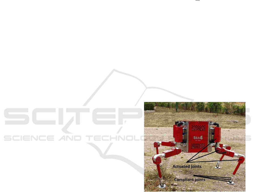
Figure 1: A leg of SILO4 walking robot (Gonzales et
al, 2003) showing its various active and passive joints.
We will apply our kinematics modeling and
control to SIL04 (Gonzales, 2003) which is a
walking robot shown in Fig. 1. SILO4 is a versatile
quadruped walking robot that has four identical legs.
Each leg has a shoulder joint, a hip and a knee joint
that are actuated. In addition, it has three passive
(compliant) joints, i.e. ankle, heel and sole that
conform to the terrain during walking. To make the
robot hybrid, we attach wheels at the leg ends, as
depicted in Fig. 2. During walking, wheels are
locked and act as feet. In the rolling mode, the
conforming foot joints are locked and the wheels are
free to rotate.
Kinematics Modelling, Optimization and Control of Hybrid Robots
119

In addition due to mechanical design of SILO4 that
is intended for walking rather than hybrid operation,
in the rolling mode the steering is performed through
the shoulder joint angle rather than at the wheel.
This makes control and path following challenging.
The four vectors mentioned in Section 4,
namely, desired
, actuated
, known
and unknown
that are used for optimization
and control are specified below for rolling and
walking of this robot.
Rolling: In this mode the desired quantities are the
trajectories of the rover body velocities which must
follow a desired path on the terrain, and thus
. The known quantity
vector
consists of wheel linear velocities which
are obtained by transforming
to the
wheel velocities
and
so as to roll the
wheels along the desired rover body trajectory. Note
that
where is the wheel radius and
are
the wheels angular velocities. Since the wheels are
constrained to be on the terrain,
is also known from
the terrain topology. We assume sensors such as laser
ranger finders or cameras are available to map the
terrain elevations in front of the robot. In addition due
to the mechanical constrains, wheel roll rate
.
The wheel pitch rate
is determined by the terrain
inclination under the wheel and is therefore known.
Finally the wheel yaw rate
is known since it must
follow the desired wheel trajectory. The actuated
quantity vector
consists of the three leg joint
angles in each of the four legs
,
. The unknown quantity vector
comprises
of the body roll, pitch and yaw rates
respectively, and the body vertical movement
, .
Walking: We assume that a planner is available that
determines the sequence of leg movements (gait
cycle). In the simulations, we use the following
sequence of leg movements: left front leg, right back
leg, right front leg, left back leg. In the above wheel
rolling, we specified the velocity trajectories of the
body
and the wheels follow these
specifications through the transformations from the
body to the wheels, making the body the leader and
the wheels followers. In walking, we specify the
trajectories of the swing leg and the body is to follow
the leg movement, i.e. the swing leg is the leader and
the body is the follower. We specify a semi-circle
path for the foot of the swing leg between its current
position on the terrain and the next point on the
desired path based on the terrain topology in front of
the robot. As mentioned before, path planning is not
the thrust of this paper. During walking the three
passive foot joints are unlocked and become
compliant (unknown). In addition the stance feet
velocities
=0 since these feet must be
fixed on the terrain.
The transition between walking and rolling takes
place using body roll
and pitch
. The transition
from rolling to walking takes place when
, and from walking to rolling when at
the time when the four feet touch the ground and
where is a threshold and is
the hysteresis width used to avoid oscillating between
rolling and walking. Alternatively a laser ranger
finder or cameras can determine the terrain topology
and decide the transition.
Figure 2: Robot on a small section of the terrain.
In order to test the performance of the kinematic
modeling and control, we consider a terrain which has
both bumps and relatively flat surfaces a small section
of which is given in given in Fig. 2. The maximum
height of bumps is cm. The desired path is chosen
to be circular with a radius of about meters
which the robot traverses in about 400 seconds,
giving the average linear speed of m/s which is
equal to fast human walk. The desired circle defines
two other circles with radii
and
where is
the width of the rover. One side of the rovers
wheels/feet is desired to traverse over the inner blue
circle in Fig. 3, and the other side is specified traverse
on the outer green circle.
The optimization criterion (17) is applied with
and
to keep
the rover balanced and maintain the legs joints with
angles close to their center ranges.
The variations of the three actuated joint angles of leg
2 are given in Fig. 4 for one full cycle, i.e. during the
time when all four legs complete their motion which
takes about 3.5 second. The joint angles variations in
the other legs, not shown due to space limitation,
exhibit similar responses. Fig. 5 shows the traces of
the body, links and joint, and feet (locked wheels) for
one cycle of walking after all four feet have gone
through their semi-circle paths. Note that at any time
ICINCO 2019 - 16th International Conference on Informatics in Control, Automation and Robotics
120
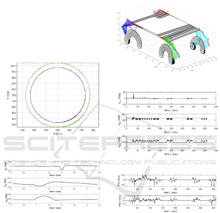
only the swing foot is moved and the other three
stance feet are stationary.
In Fig. 6 we show the joint angles in another leg,
namely leg 4, during the traversal of the whole
circular path which takes about 400 s. Note that
significant changes of joints angles take place during
walking when the robot traverses over bumps. This is
necessary to keep the rover balanced as one leg is
lifted from the ground and the body moves forward.
The periods of low angle variations in Fig. 6 are due
to wheels rolling, rather than walking, over the
relatively smooth part of the terrain.
Figure 3: The desired inner side (in blue) and outer side
(green) of the paths for the wheels/feet. The actual paths
are shown in red.
Figure 4: The variations of joints of leg 2 during one cycle
of walk.
The rover balance as reflected in the body pitch
and roll is provided in Fig. 7. It is seen that the
optimization (17) has kept the robot pitch and roll
small, with the maximum roll of about 10 degrees and
the maximum pitch of 5 degrees, essentially levelling
the robot despite variations in the terrain topology.
The traces of the desired circular paths of the inner
and outer wheels/feet are shown in Fig. 3, in green
and blue, respectively, and actual paths traversed by
the robot wheel and feet are shown on both circles in
red. It is evident that the control scheme described in
Section 4 has kept the robot very close to the desired
path with a maximum error of about 5 cm.
Figure 5: The traces of feet (locked wheels) for one cycle
after all feet have completed their trajectories.
Figure 6: Leg 4 joints angles variation during the whole
period of traversing the circular path.
Figure 7: Body pitch and roll variation during traversal of
the circular path.
6 CONCLUSIONS
Traditional approaches to kinematics modelling,
optimization and control of robots have used a variety
of different methods each suitable for a particular type
of robot. In contrast this paper has developed a
unified kinematics modelling with an embedded
optimization criterion in a form which can be applied
to almost any type of robot. The fundamental
kinematics equation of a general hybrid robot is
Kinematics Modelling, Optimization and Control of Hybrid Robots
121

presented in a compact form. This equation is then
used to derive the kinematics equations in several
useful forms such as companion, actuation,
optimization and control forms. The proposed unified
approach can be applied to various robots, including
any combination of propulsion such as hybrid
walking/rolling, mobile manipulators and Stewart-
type platforms. A software package has been
developed to implement the kinematics modelling and
optimization in its various forms. The software
includes animation of the robot motion. The program
has been applied to a hybrid walking/rolling robot for
traversing on bumpy terrain. Various results
demonstrate the satisfactory performance of the
systems in path following, balancing and tip-over
avoidance.
REFERENCES
Bellicoseo, C.D., Jenelten, F., Gehring, C. and Hutter, M.,
2018. Dynamic locomotion through online nonlinear
motion optimization for quadruped robots,” IEEE
Robotics and Automation Letters, vol. 3, no. 3, pp.
2261-2268.
Cordes, F., Dettmann, A., and Kirchner, A., 2011.
Locomotion modes for a hybrid wheeled-legplanetary
rover, in Proc. of IEEE Int. Conf. on Robotics and
Biomimetics, vol. 1, pp. 654–659, 2004.
Cully, A., Clune, J., Tarapore, D., and Mouret, J-B., 2015.
Robots that can adapt like animals,” Nature volume521,
pp. 503–507.
Gonzales de Santos, P., Estremera, J., and Garcia, E., 2003.“
The SILO4- A true walking robot for comparative study
of walking machines techniques. IEEE Robot. Autom.
Mag., vol. 10, no. 4, pp. 23- 32.
Grand, C. BenAmar, F., Plumet, F. and Bidaud, P., 2000.
Stability control of a wheel-legged mini-rover, in Proc
of Int. Conf. on Climbing and Walking Robots.
Fujita, T., and Sasaki, T., 2017. “Development of hexapod
tracked mobile robot and its hybrid locomotion with
object-carrying,” IEEE Int. Symp. on Robotics and
Intelligent Sensors.
Iagnemma, K., Rzepniewski, A., Dubowsky, S.,
Huntsberger, T., Pirjanian, P., Schenker, P., 2000.
Mobile Robot Kinematic Reconfigurability for Rough-
Terrain,” Proceedings of the SPIE Symposium on
Sensor Fusion and Decentralized Control in Robotic
Systems III.
Jehanno, J-M., Cully, A., Grand, C., and Mouret, J-B., 2014.
“Design of a wheel-legged hexapod robot for creative
adaptation,” World Scientific Publishing, vol. 20, no. 6.
Kelly, A. and Seegmiller, N. 2015 “Recursive Kinematic
Propagation for Wheeled Mobile Robots”, vol. 34, no.
3, Int. J. Robotics Research. .
Kelly, A., 2012 “A vector algebra formulation of mobile
robot velocity kinematics,” Proc. 2012 Int. Conf. Field
and Service Robots.
Muir, P.F., and Neuman, C. P., 1991. “Kinematic modeling
of wheeled mobile robots,” J. Robotic Systems vol. 4, no.
2, pp. 281–340.
Nakamura, N., 1991. Advanced Robotics-Redundancy and
Optimization, Chapter 4, Addison-Wesley.
Rajagopalan, R., 1997 “A generic kinematic formulation for
wheeled mobile robots,” Journal of Robotic Systems
vol. 14, no. 2, pp. 77–91.
Shkolnik, A. and Tedrake, R. 2007. “Inverse Kinematics for
a Point-Foot Quadruped Robot with Dynamic
Redundancy Resolution”, 2007 IEEE Int. Conf.
Robotics and Automation Roma, Italy.
Siegwart, R., Lamon, P., Estier, T., Lauria, M., and Piguet,
R., 2002. “Innovative design for wheeled locomotion in
rough terrain,” Robotics and Autonomous Systems, vo.
40, pp. 151–162.
Shin, D.D., and K.H. Park, K.H., 2001. “Velocity kinematic
modeling for wheeled mobile robots,” Proc. 2001 IEEE
Int. Conf. Robotics and Automation, vol. 4. pp. 3516–
3522.
Smith, J., Sharf, I., and M. Trentini, M., 2006. Paw: a
Hybrid wheeled-leg robot, in Proc. of IEEE Int. Conf.
on Robotics and Automation.
Tarokh, M., McDermott, G., Hayati, S., and Hung, J., 1999
"Kinematic modeling of a high mobility Mars rover,"
Proc. IEEE Int. Conf. Robotics and Automation, pp.
992-998.
Tarokh, M. and McDermott, G., 2005. Kinematics
modelling and analysis of articulated rovers. IEEE
Trans. Robotics, vol. 21, no. 4, pp. 439-454.
Tarokh, M., G. McDermott and L. Mireles, 2006. Balance
control of articulated rovers with active Suspension.
Proc. 8th IFAC-IEEE Symposium on Robot Control:
Vol. FrP- 2.1-2, pp. 1-6. Bologna, Italy.
Tarokh, M., and McDermott, G., 2007. “A systematic
approach to kinematics modeling of high mobility
wheeled rovers,” Proc. IEEE Int. Conf. Robotics and
Automation, pp. 4905- 4910, Rome, Italy.
Tarokh, M., Ho, H.D., and A. Bouloubasis, A., 2013.
Systematic kinematics analysis and balance control of
high mobility rovers over rough terrain," J. Robotics and
Autonomous Systems, 61, 13-24.
Winkler, A.W., Farshidian, F., Pardo, D., Neunert, M., and
Buchli, J., 2017. “Fast Trajectory Optimization for
Legged Robots Using Vertex-Based ZMP Constraints,”
IEEE Robotics and Automation Letters, Vol. 2, No. 4,
pp.2201-2208.
Winkler, A.W., Bellicoso, C.D., Hutter, M. and J. Buchli, J.,
2018. “Gait and trajectory optimization for legged
systems through phased-based end-effector
parameterization,” IEEE Robotics and Automation
Letters, vol.3, no. 3, pp. 1560-1567.
Ylonen, S., and Halme, A., 2002. Further development and
testing of the hybrid locomotion of Workpartner robot,
in Proc of Int. Conf. on Climbing on Walking Robots
(CLAWAR).
Yuan, J., and S. Hirose, S., 2004. “Research on leg-wheel
hybrid stair- climbing robot,zero carrier,” in IEEE Int.
Conf. on Robotics and Biomimetics.
ICINCO 2019 - 16th International Conference on Informatics in Control, Automation and Robotics
122

Zhong, G., Deng, H., Xin, G., and. Wang, G., 2016.
Dynamic Hybrid Control of a Hexapod Walking Robot:
Experimental Verification,” IEEE Trans. Industrial
Electronics, , Vol. 63, No. 8. pp.5001-5011.
Kinematics Modelling, Optimization and Control of Hybrid Robots
123
