
Time Synchronisation of Low-cost Camera Images with IMU Data based
on Similar Motion
Peter Aerts and Eric Demeester
ACRO Research Group, Department of Mechanical Engineering, University of Leuven, Diepenbeek, Belgium
Keywords:
Time Synchronisation, Particle Filter, Clock Parameter Estimation, Camera/IMU Synchronisation.
Abstract:
Clock synchronisation between sensors plays a key role in applications such as in autonomous robot navigation
and mobile robot mapping. Such robots are often equipped with cameras for gathering visual information. In
this work, we address the problem of synchronizing visual data collected from a low-cost 2D camera, with
IMU (Inertial Measurement Unit) data. Both sensors are assumed to be attached to the same rigid body;
hence, their motion is correlated. We present a motion based approach using a particle filter to estimate the
clock parameters of the camera with the IMU clock as a reference. We apply the Lucas-Kanade optical flow
method to calculate the movements of the camera in its horizontal plane corresponding to its recorded images.
These movements are correlated to the motion registered by the IMU. This match allows a particle filter to
determine the camera clock parameters in the IMU’s time frame and are used to calculate the timestamps of
the images. We presume that only the IMU sensor provides timestamp data generated from its internal clock.
Our experiments show that given enough features are present within the images, this approach has the ability
to provide the image timestamps within the IMU’s time frame.
1 INTRODUCTION
In the field of autonomous robotics, it is important
that the robot consistently interprets its environment
and timely reacts to situations such as avoiding col-
lisions. Various sensor types are typically adopted in
order to collect different types of data to achieve this
interpretation. A main aspect in mobile robotics and
autonomous navigation is position estimation which
plays a key role in the proper execution of tasks. Fus-
ing data from different sensors allows to estimate the
positions and actions of these autonomous robots. An
important aspect of sensor fusion is time synchroniza-
tion between sensors. In order to optimize the combi-
nation of different datasets, knowledge regarding the
instants at which the data were obtained is paramount.
The use of cameras and computer vision is becoming
an important part in the field of robotics. For instance
in vision perception for mobile platforms (Horst and
Moller, 2017). This paper focuses on synchronizing
images of a low-cost 2D camera with movement data
obtained from an IMU (Inertial Measurement Unit).
These low-cost cameras often do not provide times-
tamp information with their images due to the lack of
embedded hardware, nor can they be triggered with
an external signal. For many of these sensors a soft-
ware generated timestamp is adopted, which is based
on the internal clock of the computer and the arrival
time of the recorded image. Many publications on
sensor synchronization exist, clearly showing the im-
portance of this topic. Most approaches search for the
clock offset between two clocks and clock skew. (Wu
and Xiong, 2018) published a framework for multi-
sensor soft time synchronization using the Robot Op-
erating System (ROS) middleware. Their framework
generates an arranged dataset of all data based on each
individual data timestamp. They access all data in a
single node. The synchronizer takes the data queue of
lowest frequency as the baseline. For every data on
the baseline queue, it takes the nearest data on other
data queues of other sensors to join the set, resulting
in a synchronized data set. This approach assumes
that every data timestamp is accurate, ignoring pos-
sible errors of the timestamp. Assuming the data are
timestamped, (Nelsson and Handel, 2010) propose to
obtain the true timestamps using a Kalman filter based
on the sampling instances each sensor model pro-
vides. Their approach to time synchronisation is by
292
Aerts, P. and Demeester, E.
Time Synchronisation of Low-cost Camera Images with IMU Data based on Similar Motion.
DOI: 10.5220/0007837602920299
In Proceedings of the 16th International Conference on Informatics in Control, Automation and Robotics (ICINCO 2019), pages 292-299
ISBN: 978-989-758-380-3
Copyright
c
2019 by SCITEPRESS – Science and Technology Publications, Lda. All rights reserved

linear filtering the timestamps given to each measure-
ment. (Li and Mourikis, 2014) focus on the temporal
synchronization specifically between camera images
and IMU data. They present an Extended Kalman Fil-
ter (EKF) approach for online estimation of time off-
set which is included in the EKF state vector. How-
ever, their approach also assumes that the IMU and
image data are both timestamped. (Guo et al., 2015)
propose to synchronize wireless network data using
Rao-Blackwellized particle filtering(RBPF) based on
the Dirichlet process mixture (DPM) model. Their
approach estimates the clock offset and skew using
the RBPF algorithm which is based on two way tim-
ing message exchange and the DPM model to de-
scribe the noise. (Ling et al., 2018) propose a non-
linear approach to model the varying camera and IMU
time offset in order to achieve better Visual Inertial
Odometry. Their approach models the time offset
as an unknown variable to deal with an imperfect
camera-IMU synchronization. In our approach, we
assume that the images received from a low-cost cam-
era do not have a timestamp generated in hardware or
software. We propose to estimate the clock parame-
ters of the camera with which to timestamp each im-
age with respect to the time frame of an IMU’s in-
ternal clock. The contribution of this approach is to
achieve synchronization based on the same motion
that each sensor, attached to the same rigid body, ex-
periences. This approach differs from the previous
methods by not relying on the synchronization of in-
dividual sensor generated timestamps. We adopt the
following assumptions:
1. Camera and IMU are fixed to the same rigid body;
this rigid body is in motion.
2. The IMU has an internal clock and has a higher
data publishing rate in comparison with the cam-
era.
3. The images are taken at a relatively fixed fre-
quency meaning that the FPS of the camera does
not rapidly decline unawares. The focal point of
the camera is fixed, meaning that the camera is not
allowed to auto adjust its focus.
4. The environment is assumed to be static.
All hardware used in our experiments was compliant
with these assumptions. The continuation of this pa-
per is divided as follows; Section 2 covers our ap-
proach to calculate the camera movements and to es-
timate the clock parameters using the particle filter-
ing technique. In section 3 we report the results of
our experiments executed with the use of online data
streams in an indoor environment. This section is fol-
lowed by our conclusion in section 4. In section 5
we mention opportunities to further optimize our ap-
proach.
2 METHOD
In this section we present a short overview of our ap-
proach followed by the used method for determining
the movements of the 2D camera. Next, the process
of correlating the cameras movements with the move-
ments of the IMU is presented. The section closes
with the particle filter approach to estimate the clock
parameters of the camera w.r.t. the IMU’s internal
clock.
2.1 Overview
In order to estimate the moment a given image was
recorded in accordance with the IMU’s motion data,
several calculations must occur. We propose to esti-
mate the clock parameters of the camera rather than
the timestamp of each image individually. These pa-
rameters, defined as clock offset and fps (frames per
second or frame rate), can be used to estimate the
timestamps of several consecutive images. Ideally,
these parameters would be calculated for each image
individually. However, in case our program would ex-
perience lag due to the data transfer rate and the com-
putational load, consecutive images can be skipped
during the calculation process. The timestamps of
these skipped images can then be estimated with the
last known clock parameters (1).
t
img
= t
o f f set
+ f rame_rate ∗ID
img
(1)
The estimation of these parameters is calculated us-
ing a particle filter. This approach has the advantage
of being a multi-hypothesis approach. This allows us
to handle estimating the parameters in case the frame
rate of the camera exhibits slight variations. As input
for the particle filter, correlated data of the IMU and
camera must be provided. Therefore, we match the
movements of the IMU in the horizontal plane with
the movements of the camera in the same plane.
Figure 1 shows the general workflow of our ap-
proach. Three main branches are present. The ‘IMU
data’ branch collects the rotation data of the IMU
while the ‘Optical Flow’ branch collects the images
and calculates the 3D rotation and translation of the
camera using optical flow. For further calculations,
only the rotation in the horizontal plane is used. The
Time Synchronisation of Low-cost Camera Images with IMU Data based on Similar Motion
293

Figure 1: Overview of our time synchronization algorithm.
The three main branches are run as a thread. The IMU
data and Optical Flow branch each provides the motion data
streams experienced by there respective sensors. The main
branch assesses the correlation between these data streams
and runs the particle filter to estimate the clock parameters.
‘Main’ branch uses these two data streams to esti-
mate the clock parameters of the camera in the IMU’s
time frame using a particle filter. To prevent loss of
data and reduce the computation time, each of these
branches is run as a thread. This allows for the si-
multaneous computation of the camera movements
and collecting the IMU data as well as matching the
movements between the images and the IMU and es-
timating the parameters. The upcoming sections will
go further into detail of each branch.
2.2 Camera Movements
This section describes the method used to calculate
the movements of the camera. For this, we need two
sets of data 1) describing the location of trackable pix-
els within each frame 2) representing the same pix-
els in the second consecutive image. This informa-
tion can be used to calculate the rotation and trans-
lation matrix of which the former is to our interest.
The necessary data can be acquired using the Lucas-
Kanade optical flow method. However, the optical
flow method depends on three main inputs:
1. It requires the intrinsic parameters of the cam-
era. These parameters describe the position of
the camera’s focal point, the optical center and the
distortion coefficients of the camera.
2. A dataset of trackable pixels is needed as a start-
ing point to determine the two data sets of consec-
utive pixels.
3. The algorithm requires two consecutive images of
which the first image corresponds with the second
requirement.
Using the chess board calibration method avail-
able in the open source library OpenCV based on
(Zhang, 2000), the intrinsic parameters of the camera
are determined based on the pinhole camera model.
These parameters are represented as a camera matrix:
Camera =
f
x
0 c
x
0 f
y
c
y
0 0 1
Where f
x
and f
y
represent the focal point distance and
c
x
and c
y
represent the optical center location. The
intrinsic distortion parameters are represented as five
values also known as distortion coefficients:
Distortion coe f f icients = (k
1
, k
2
, p
1
, p
2
, k
3
)
These intrinsic parameters allow for compensation of
the image distortion. OpenCV also provides the tools
for determining tracking points. As previously men-
tioned, we need a starting point of the pixels to track
in order to calculate the position of these pixels within
the consecutive image. This data set can be calcu-
lated using the FAST (Features from Accelerated Seg-
ment Test) feature detection (Rosten and Drummond,
2006) (Rosten et al., 2010). This feature detector was
chosen because of its calculation speed, which allows
to determine tracking points in real time. By using
FAST, a pixel is considered to be a tracking point
within the grayscaled image when a number of the
surrounding 16 pixels’ intensities are above a certain
threshold. Written as a set of conditions (2,3):
A set of N pixels S, ∀ a ∈ S, I
a
> I
p
+t (2)
A set of N pixels S, ∀ a ∈ S, I
a
< I
p
−t (3)
Where I
p
equals the intensity of the pixel of in-
terest, I
a
represents the intensity of the surrounding
pixel and t a threshold parameter. If the amount of
pixels which meet one of these conditions is above a
certain quantity, the pixel of interest is considered a
trackable pixel. Once these trackable pixels are deter-
mined, they are used as a starting point for the optical
flow method. The Lucas-Kanade optical flow method
takes a 3x3 pixel matrix around a point of interest.
It assumes that pixel intensities do not change be-
tween consecutive images and the neighbouring pix-
els have similar motion. It solves the basic optical
flow equations (5) for these points using the least
squares method:
∂I
∂x
∗V
x
+
∂I
∂y
∗V
y
+
∂I
∂t
= 0 (4)
I
x
∗V
x
+ I
y
∗V
y
= −I
t
(5)
V
x
and V
y
are the velocity components in their re-
spective directions within the image. I
x
, I
y
and I
t
are the derivatives of the pixel intensity at instance
ICINCO 2019 - 16th International Conference on Informatics in Control, Automation and Robotics
294

(x, y,t) where x and y represent the pixel location and
t its time instance. By solving the basic optical flow
equations, the Lucas-Kanade optical flow function is
able to determine the location of the feature points
within the next image with the assumption that the
movement between the consecutive images is rela-
tively small. These new locations are also used as
the input for the next optical flow calculation. Only
if the number of trackable pixels or feature points de-
clines below a certain threshold, the FAST feature de-
tection is reapplied. This limits the computational
load of the algorithm by avoiding constant feature
point determination. The algorithm requires a mini-
mum of 5 point pairs between two consecutive images
for further calculation. This by itself sets the min-
imum threshold for reapplying the feature detection
to 5 feature points. Once the two data sets are avail-
able (the feature points within the two consecutive im-
ages), the rotation matrix can be calculated. First, the
essential matrix from the corresponding points within
the two images is to be determined. The RANSAC
method is used for computing the fundamental ma-
trix. Using this matrix, the essential matrix is esti-
mated based on the five-point algorithm described in
(Nister, 2003). Once the essential matrix is estimated,
the rotations and translations are calculated (Malis
and Vargas, 2007) and their feasibility is checked us-
ing a cheirality check (Nister, 2003). This check ver-
ifies the possible pose estimations by analyzing if the
triangulated 3D points have positive depth within the
two consecutive images. Once the rotation matrix is
obtained the values are converted to Euler angles.
2.3 Correlating Camera and IMU Data
to Find Time Shift
The previous section described how the movements of
the camera are acquired. Simultaneously, data from
an IMU are collected, of which the Euler angles are
used. In our case, we selected only the Euler angle
in the horizontal plane for further calculations. The
data of the IMU together with its provided timestamp
are written to a dynamic list. Within this list, old data
is discarded when new data is available. The image
ID together with the movements obtained using the
Lucas-Kanade optical flow method is similarly writ-
ten to a dynamic list. A maximum number of data
points is set on the IMU list. Once the amount of data
within the IMU list reaches this threshold, the amount
of data gathered in the camera list, which runs paral-
lel with gathering the IMU data, is set as its treshold.
Data is continuously written and discarded within the
lists. Due to the frequency of the IMU being much
higher than the frame rate of the camera, a linear in-
terpolation is applied to the rotation data of the cam-
era. After this step, the data of both sensors are nor-
malized. Once normalized, a cross-correlation is per-
formed between the two data sets. Algorithm 1 pro-
vides the pseudo code for this approach.
DATA: rotation matrix camera: R_{cam},
yaw rotation: y_{cam}, y_{imu},
lists: Y_{cam}, Y_{imu}
RESULT: Correlation between IMU and
camera motion:Corr
for Y_{imu} to Threshold step 1 do:
Fill list Y_{imu}=Y_{imu} + <y_{imu}>;
if R_{cam}=new R_{cam} then:
y_{cam}=get_Euler_Angle_YAW(R_{cam};
Y_{cam}=Y_{cam}+ <y_{cam}>;
end
if y_{imu}=new y_imu then:
Y_{imu}=Y_{imu} - <y_{imu(0)}>
+ <new y_{imu}>;
if y_{cam}=new y_{cam} then:
Y_{cam}=Y_{cam} - <y_{cam(0)}>
+ <new y_{cam}>;
Y_{cam}=interpolat[Y_{imu},Y_{cam}];
Y_{imu}=normalize[Y_{imu}];
Y_{cam}=normalize[Y_{cam}];
corr=cross_Corr[Y_{imu}, Y_{cam}];
return corr;
end
end
end
Algorithm 1: Pseudo code for matching movement data.
Visualized in figure 1 as part of the main branch. Rota-
tion data y
imu
and y
cam
are added to the lists Y
imu
and Y
cam
.
When new IMU data arrives and is added to the list, the
oldest data is discarded. Each time new IMU data is avail-
able, we check if there is also new camera movement data
available. Once both lists contain the most current informa-
tion, the lists are interpolated, normalised and a correlation
is preformed between the two movements.
The correlation function in our approach origi-
nates from the SciPy library in Python. The cross-
correlation allows the algorithm to match the latest
incoming image to a time stamp in accordance with
one of the data points provided by the IMU.
Time Synchronisation of Low-cost Camera Images with IMU Data based on Similar Motion
295

2.4 Estimating the Clock Parameters
Using cross-correlation to find the time shift between
camera rotation and IMU rotation still does not pro-
vide the clock parameters of the camera. We need
these clock parameters, because once they are known,
we can calculate the timestamps for every image. To
estimate the clock offset and frame rate, a particle fil-
ter is implemented. This filter allows to consider mul-
tiple clock hypotheses. When there is a slight vari-
ance in the frames per second, the algorithm will be
able to deal with these changes accordingly due to its
multi-hypothesis approach. Dependent on the num-
ber of hypotheses (or particles) used, the particle fil-
ter will convert to the best estimated parameters more
quickly. The filter is described as pseudo code in Al-
gorithm 2.
DATA: particles:x_{t} elem of X_{t}
action:u_{t}, measurement:z_{t},
weight:w_{t}
RESULT: particles:X_{t},
best particle:x_{max}
for m=size{X_{t}} to num_of_particles
step 1 do:
sample for instance m
x_{t} = p(x_{t}|u_{t},x_{t-1});
calculate weight for instance m
w_{t}=p(z_{t}|x_{t});
Z_{t} = Z_{t}+<x_{t},w_{t}>;
end
for m=0 to elements in Z_{t}
step 1 do:
draw particle for instance m
x_{t} where w_{t}>w_{mean};
X_{t} = X_{t} + <x_{t}>;
draw particle x_{max} where
w_{max}=max(w_{t});
return X_{t}, x_{max};
end
Algorithm 2: Particle filter to estimate clock parameters.
One of the branches visualized in figure 1. A set of parti-
cles is created with clock parameters. They are assigned
a weight and added to the list Z
t
. The particles with a
weight higher than the mean weight of all current particles
are maintained. These are added to the list X
t
.
Z
t
represents the list of particles X
t
at a given time
t −1. Another input of the filter is u
t
which represents
the recent action. In our case, it betokens the moment
a new image is available represented by the image ID.
When the particle filter is called for the first time, all
particles are created with random guessed offset and
frame rate around a given start value. The initial guess
of the offset estimation is given by the first timestamp
of the IMU data received at the starting point. The
frame rate parameter randomly distributes around the
ideal frame rate (30 fps). When the particle filter is
repeatedly called, each particle is updated according
to the image ID. Every particle provides a timestamp
based on its parameters. Depending on the weight w
t
some particles are discarded and are recreated with
random parameters when an update occurs. If the
weight of a particle is high enough, the hypothesis
is maintained. This weight of each particle changes
with every update. z
t
represents the timestamp of the
correlated data which were obtained by matching the
movements of the camera with the IMU. This input
is used to calculate the weight of each particle or hy-
pothesis. In our particle filter, the weights of each par-
ticle are calculated based on the Gaussian distribution
function:
w =
1
σ
√
2π
e
−(x−z)
2
.
2σ
2
(6)
Where w represents the calculated weight with σ
2
be-
ing the set variance. The variables x and z represent
the estimated timestamp of the hypothesis and the
IMU timestamp respectively. When each hypothesis
has been assigned a weight, the values are normalized.
w
n
=
w
p
p
∑
i=0
w
i
(7)
w
n
represents the normalized weight based on the
original weight of the hypothesis (w
p
) divided by the
sum of the weight of all p hypotheses. After this nor-
malization step, a selection of particles is made which
we assume to best approximate the clock parameters.
This selection is set at the median of all particles. This
means we maintain fifty percent of all hypotheses for
our next update of the particle filter. The other hy-
potheses are discarded and new hypotheses are cre-
ated as a replacement. The parameters of these new
clock hypotheses are randomly attributed around the
parameters of the particle with the highest normalized
weight. This allows the algorithm to converge to the
correct parameters at a higher rate. Consequently, we
assume that the particle with the highest weight has
the highest probability of being correct and thus rep-
resents the optimal clock parameters. These parame-
ters are used to calculate the timestamps of the images
up to the point that the particle filter is executed once
more.
ICINCO 2019 - 16th International Conference on Informatics in Control, Automation and Robotics
296
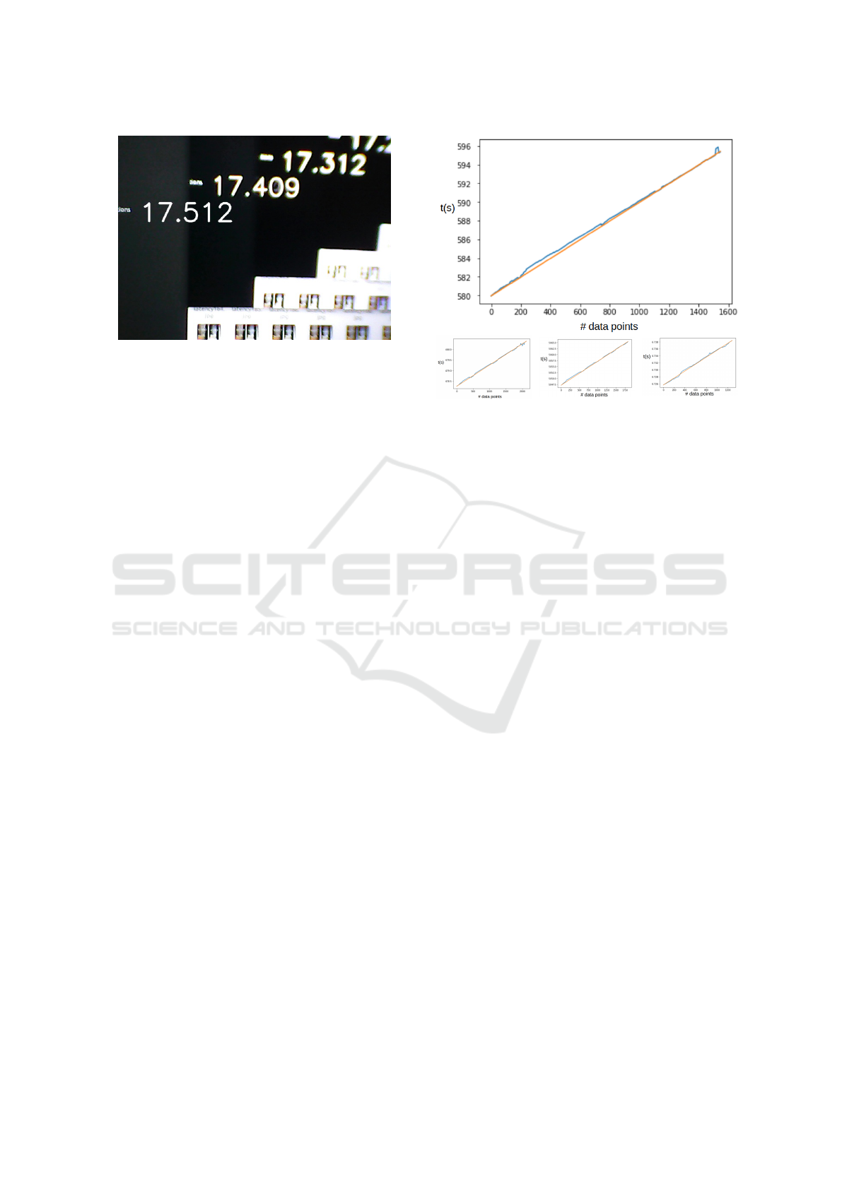
Figure 2: Two consecutive images replayed from the cam-
era with their timestamp. The difference between the two
consecutive images defines the latency. Time is given in
seconds.
3 EXPERIMENTS
In this section we share the results of our conducted
experiments and the difficulties we encountered. The
outcome of our time synchronization program which
is written in Python 3.6., is a list of camera im-
age timestamps and IMU timestamps. We aimed to
achieve the synchronisation of an XSENS Mti-G-710
IMU with an ICIDU VI-707801 webcam. The im-
ages produced by the CMOS camera can directly be
accessed in Python using OpenCV. The IMU was cal-
ibrated using the delivered software by XSens. This
software package allowed us to format the data output
to publish Euler angles and timestamps. After this,
using a Python written driver, we read in the correct
data in order to estimate the webcam’s clock param-
eters and consequently to estimate each image time
stamp using our algorithm. As a baseline and prof-
itability check, we ascertained the latency of the we-
bcam. A script was written in OpenCV to read in
the webcam images and to publish a timestamp on
the screen of the laptop. This timestamp is gener-
ated with the clock of the computer. When the screen
is recorded, the current timestamp is being published
and captured within the image of the camera. This im-
age is shown on the screen of the computer. The next
recorded frame has the new timestamp of the com-
puter as well as the previous frame with its timestamp,
see figure 2. Take note that the time displayed is set
in seconds.
The difference between the time shown on the
screen and the time displayed in the image from the
USB camera is considered to be the latency of the
camera. In our case, the mean latency of our web-
Figure 3: Timestamp comparison graphs: IMU constant
publishing rate plotted with estimated camera timestamps.
cam is 91 ms calculated from 100 images. The aver-
age FPS of the webcam is 29 frames per second. We
also noticed that a significant change in light inten-
sity impacts the frame rate. Under normal light con-
ditions, the camera frame rate is relatively constant at
29 frames per second. However, in environments with
low light intensity, the frame rate descended drasti-
cally to an average of 10 frames per second. The IMU
was set to publish data every 10 milliseconds (100 Hz)
including its own timestamp. The threshold for the
number of elements in the IMU data list was set to 40
data points. The number of particles produced by the
particle filter was set to 1000 to achieve a good esti-
mate more quickly. Figure 3 shows the timestamps of
the IMU plotted for each data point in orange. The
timestamps of the camera images are plotted in blue.
In ideal conditions, due to the correlation between the
movements of the two sensors, these two lines would
fully coincide. In our results, we can see that the
timestamps follow the same linearity and no major de-
viation occurred during our synchronization. Several
runs were conducted with similar results.
Using correlation to estimate the clock parameters
resulted in timestamping the images based on their
movement. To eliminate the latency which is aver-
aged at 91 ms should the images receive a timestamp
at their point of arrival. Take into account that the la-
tency of the images varies due to the low-cost/quality
ratio of the webcam. Several runs were conducted and
checked against the linearity of the IMU timestamps.
Our results show that a mean deviation of 44 ms oc-
curred. In some runs the deviation was 15 ms between
the IMU timestamps and image timestamps, effec-
Time Synchronisation of Low-cost Camera Images with IMU Data based on Similar Motion
297

tively showing that this method can approximate the
time an image was taken based on correlated move-
ment. However, notice that there are some irregular-
ities within the graph of the image timestamps and
that the linearity is not constantly preserved. This
has several possible causes. For one, the algorithm is
written to synchronize low-cost cameras having a rel-
atively stable frame rate. However, if this frame rate
changes rapidly, the particle filter needs time to adjust
to a large difference. As previously mentioned, ex-
treme changes in light conditions can affect the frame
rate substantially. Second, fast movements may cre-
ate blurry images. This makes tracking pixels of inter-
est to determine the camera movements troublesome.
Third, a lack of features within an image makes cam-
era motion determination challenging.
4 CONCLUSION
We presented a new synchronization approach to syn-
chronize images, which lack timestamps, of a low-
cost camera with IMU data based on similar move-
ment. Our approach assumes that the IMU publishes
a timestamp generated with its internal hardware. We
also assume that the camera has a relatively stable
frame rate whithout a changing focal point of the cam-
era lens. In our approach, a particle filter is used to
estimate the clock parameters (offset and fps) of the
camera, which allows for multiple hypotheses. This
makes it possible to manage slight changes in the
camera’s frame rate. These slight changes are de-
pendent on the camera hardware and its behaviour
towards external factors such as large light intensity
variations. The results show that this approach can
effectively synchronize the recorded images with the
IMU data within the IMU’s time frame under optimal
conditions. The approach reduces the timestamp error
of the images in comparison with the latency, show-
ing that we can reduce the timestamp error of soft-
ware generated timestamps. However, some difficul-
ties can arise during the synchronisation process. Ex-
ternal factors such as movement speed, lighting con-
ditions, and environmental aspects affect the quality
of the images. This creates difficulties for calculating
the optical flow.
5 FUTURE WORK
Some improvements to our current approach are fea-
sible; Firstly, the algorithm can be further extended by
correlating movements in 3D space instead of the cur-
rent 2D space method. While our 2D space method is
useful for mobile robots and other wheel driven ap-
plications operating in a horizontal plane, 3D space
expands the synchronisation approach to almost all
robotic applications using camera’s and IMU’s. Sec-
ondly, increasing the amount of data points by inter-
polating the data sets of the camera movements and
IMU movements could improve the accuracy of the
correlation. This in turn can improve the synchroniza-
tion algorithm. However, adding more computational
load to the algorithm could have counterproductive
results. Finally, the camera used in our experiments
provides low quality images. Higher quality images
may improve the optical flow calculation and provide
better rotation estimations.
ACKNOWLEDGMENT
Peter Aerts is an SB PhD fellow at FWO (Re-
search Foundation Flanders) under grant agreement
1S67218N.
REFERENCES
Guo, C., Shen, J., Sun, Y., and Ying, N. (2015). Rb parti-
cle filter time synchronization algorithm based on the
dpm model. In in Sensors, 15(9), 22249-22265.
Horst, M. and Moller, R. (2017). Visual place recognition
for autonomous mobile robots. In Robotics, 6(2), 9.
Li, M. and Mourikis, A. (2014). Li, m. and mourikis, a.
i. (2014). online temporal calibration for camera-imu
systems: Theory and algorithms. In The International
Journal of Robotics Research, 33(7), 947-964.
Ling, Y., Bao, L., Jie, Z., Zhu, F., Li, Z., Tang, S., Liu,
Y., Liu, W., and Zhang, T. (2018). Modeling varying
camera-imu time offset in optimization-based visual-
inertial odometry. In In Proceedings of the European
Conference on Computer Vision (ECCV) (pp. 484-
500).
Malis, E. and Vargas, M. (2007). Deeper understanding of
the homography decomposition for vision-based con-
trol. In (Doctoral dissertation, INRIA).
Nelsson, J. and Handel, P. (2010). Time synchronisation
and temporal ordering of asynchronous sensor mea-
surements of a multi-sensor navigation system. In In
IEEE/ION Position, Location and Navigation Sympo-
sium (pp. 897-902). IEEE.
Nister, D. (2003). An efficient solution to the five-point rela-
tive pose problem. In In 2003 IEEE Computer Society
Conference on Computer Vision and Pattern Recogni-
tion,.
ICINCO 2019 - 16th International Conference on Informatics in Control, Automation and Robotics
298

Rosten, E. and Drummond, T. (2006). Machine learning
for high-speed corner detection. In In European con-
ference on computer vision (pp. 430-443). Springer,
Berlin, Heidelberg.
Rosten, E., Porter, R., and Drummond, T. (2010). Faster
and better: A machine learning approach to corner de-
tection. In IEEE transactions on pattern analysis and
machine intelligence, 32(1),.
Wu, J. and Xiong, Z. (2018). A soft time synchronization
framework for multi-sensors in autonomous localiza-
tion and navigation/. In In 2018 IEEE/ASME Inter-
national Conference on Advanced Intelligent Mecha-
tronics (AIM) (pp. 694-699).
Zhang, Z. (2000). A flexible new technique for camera cali-
bration. In IEEE Transactions on pattern analysis and
machine intelligence, 22.
Time Synchronisation of Low-cost Camera Images with IMU Data based on Similar Motion
299
