
Modeling of Passenger Demand using Mixture of Poisson Components
Matej Petrou
ˇ
s
1,2
, Ev
ˇ
zenie Suzdaleva
1
and Ivan Nagy
1,2
1
Department of Signal Processing, The Czech Academy of Sciences, Institute of Information Theory and Automation,
Pod vod
´
arenskou v
ˇ
e
ˇ
z
´
ı 4, 18208 Prague, Czech Republic
2
Faculty of Transportation Sciences, Czech Technical University, Na Florenci 25, 11000 Prague, Czech Republic
Keywords:
Mixture Estimation, Poisson Components, Passenger Demand.
Abstract:
The paper deals with the problem of modeling the passenger demand in the tram transportation network. The
passenger demand on the individual tram stops is naturally influenced by the number of boarding and disem-
barking passengers, whose measuring is expensive and therefore they should be modeled and predicted. A
mixture of Poisson components with the dynamic pointer estimated by recursive Bayesian estimation algo-
rithms is used to describe the mentioned variables, while their prediction is solved with the help of the Poisson
regression. The main contributions of the presented approach are: (i) the model of the number of boarding
and disembarking passengers; (ii) the real-time data incorporation into the model; (iii) the recursive estimation
algorithm with the normal approximation of the proximity function. The results of experiments with real data
and the comparison with theoretical counterparts are demonstrated.
1 INTRODUCTION
The paper deals with the problem of modeling the
passenger demand in the tram network, which is an
important task in the public transportation. In order
to provide a high-quality and attractive public trans-
port service, it is necessary to minimize the number of
overcrowded vehicles. Moreover, in order to provide
economically effective service and to reduce human
resources needed, it is also necessary to minimize the
number of insufficiently occupied vehicles.
In this area, many papers deal with the passenger
demand models in metro systems (Sun et al., 2015;
Roos et al., 2016; Sun et al., 2015(a)). They use data
from turnstiles both at the entrance and the exit at
stations, which could be paired for passengers using
smart cards. In this case, continuous measurements
of the passenger flow are available. However, for ex-
ample, in central Europe, most metro networks are so
called ”open networks” without turnstiles and there-
fore without continuous measuring of the passenger
demand, which means it should be modeled and pre-
dicted. Aside from metro systems, methods of the
demand modeling have been also investigated for bus
networks (Samaras, 2015; Bai et al., 2017; Lijuan and
Chen, 2017; Ma et al., 2014), where continuous mea-
suring of the passenger demand is an expensive task
as well as in tram networks. For tram transportation,
the thesis (Pu
ˇ
sman, 2013) proposed a method of pro-
portional transit division (PTD) using deterministic
models for the passenger demand calculation.
Generally, the approaches in the discussed field
are based on: (i) regression models, (ii) artificial
neural networks or (iii) hybrid models combining
them. For example, (Milenkovi
ˇ
c et al., 2016) pro-
posed seasonal autoregressive integrated moving av-
erage model to be used on Serbian railways. (Zhou
et al., 2013) introduced three different models of the
passenger demand in bus networks. The first one was
a time varying Poisson model. Secondly, a weighted
time varying Poisson model was proposed to cope
with irregularities in passenger demand. Finally, an
autoregressive integrated moving average model was
also proposed in this paper. All three models were
applied for data from buses in Yantai, China with the
final model achieving the most accurate results.
In the area of artificial neural networks, the fol-
lowing papers were found. (Chen and Wei, 2011)
used back-propagation neural networks for the pas-
senger demand description in the Taipei metro sys-
tem. (Tsai et al., 2009) dealt with two neural net-
work models in the Taiwan railway network. The first
one was the multiple temporal units neural network
and the second was parallel ensemble neural network.
The latter provided more accurate results. (Bai et al.,
2017) introduced deep belief networks for the passen-
Petrouš, M., Suzdaleva, E. and Nagy, I.
Modeling of Passenger Demand using Mixture of Poisson Components.
DOI: 10.5220/0007831306170624
In Proceedings of the 16th International Conference on Informatics in Control, Automation and Robotics (ICINCO 2019), pages 617-624
ISBN: 978-989-758-380-3
Copyright
c
2019 by SCITEPRESS – Science and Technology Publications, Lda. All rights reserved
617

ger flow prediction on a bus line.
A series of studies combine more models to adapt
them to their specific tasks. (Lijuan and Chen, 2017)
combined stacked auto-encoder (SAE) and deep neu-
ral network (DNN) into SAE-DNN model for the
passenger demand prediction in the Xiamen bus sys-
tem. (Sun et al., 2015) proposed a combination of
wavelet transformation and support vector machine
models in the Beijing subway system. (Jiang et al.,
2014) focused on the empirical mode decomposition
(EEMD) and grey support vector machine (GSVM)
hybrid model of the passenger demand in the high-
speed railway network in China.
Besides methods mentioned above, other ap-
proaches have also been used, e.g., Bayesian net-
works (Roos et al., 2016; Sun et al., 2015(a)), stochas-
tic hybrid automat and Petri nets (Haar and Theissing,
2016) and others.
Despite the significant number of studies, current
methods possess a series of disadvantages, such as,
e.g., narrow specification, fluctuations in predictions,
etc. Analyzing the above state of the art, it can be
stated that the problem of demand modeling still calls
for novel reliable solutions.
The presented approach is based on the definition
of the passenger demand at a tram stop as the number
of passengers currently using a tram vehicle at a time
moment. Since the vehicle occupancy can change
only at stops, it is determined by adding the number
of boarding passengers and subtracting the number of
disembarking passengers at each stop, i.e.,
demand = current demand − disembarking +boarding.
However, measuring the number of boarding and
disembarking passengers in the tram network is still
a complicated task, and such measurements are not
available without specific surveys. Thus, these vari-
ables should be modeled and predicted as well. They
will create the basis for the prediction of the demand.
This paper proposes a novel approach to the mod-
eling of the passenger demand in the tram transporta-
tion network using a mixture of Poisson components
with the dynamic pointer estimated using recursive
Bayesian algorithms primarily based on (K
´
arn
´
y et al.,
1998; Peterka, 1981; K
´
arn
´
y et al., 2006; Nagy and
Suzdaleva, 2017). The approach is represented in two
parts, where the first one deals with the available data
set used for the recursive estimation of the model, and
the second one uses the estimated model for the pre-
diction. The approach is demonstrated for the number
of boarding passengers.
The layout of the paper is organized as follows.
Section 2 introduces the models used and specifies the
problem. Section 3 proposes a recursive algorithm
of the Bayesian estimation, which represents the first
part of the proposed approach. Section 4 is devoted to
the prediction part of the presented solution. Results
of experiments with real data and the discussion are
demonstrated in Section 5. Conclusions can be found
in Section 6.
2 MODELS
Let’s observe a system, which represents a tram line,
consisting of n
s
stops. The individual tram trips de-
part from each stop at non regularly discretized time
periods. In this work, the time of trip departures will
be used as discrete instants of time corresponding to
realizations of random variables and will be denoted
by the index t. At each stop s ∈ {1, 2, . . ., n
s
}, the sys-
tem generates the number of passengers boarding the
tram trip t, which is denoted by y
b
s;t
and similarly, the
number of disembarking passengers y
d
s;t
.
Having, e.g., three following stops s
1
, s
2
and s
3
,
the passenger demand denoted by D
23;t
between stops
s
2
and s
3
for a trip t is defined as:
D
23;t
= D
12;t
− y
d
2;t
+ y
b
2;t
. (1)
Let’s assume that for each stop s the variables y
d
s;t
and
y
b
s;t
can be measured for trips t = {1, 2,. . . , T } and are
no longer available for t > T .
In order to be able to use equation (1) recursively
for a line consisting of n
s
stops, it is necessary to de-
scribe firstly the number of boarding (similarly dis-
embarking) passengers at a single stop. Here, for the
sake of simplicity the approach will be shown for the
number of boarding passengers y
b
s;t
. In the case of dis-
embarking passengers, the approach will be the same.
Thus, for the better transparency of the approach, the
superscripts b and d will be omitted.
The available data set of the variables y
s;t
can be
used as the prior knowledge for the preliminary analy-
sis for a choice of the model probability density func-
tion (pdf). Based on the visual analysis of histograms
of the number of boarding passengers at stops in the
considered tram lines, the Poisson distribution as the
discrete distribution with high finite number of possi-
ble values suitable for non-negative data was chosen
for the description of the data. The example of the
histogram at a selected stop is shown in Figure 1.
In addition, the figure shows that the variables
are of the multimodal nature. This can be explained
by the behavior of passengers changing probably ac-
cording to a day period, e.g., morning peak time,
lunchtime, afternoon peak time, etc. It means that for
the description of the number of boarding passengers,
a mixture of Poisson pdfs can be a suitable tool.
ICINCO 2019 - 16th International Conference on Informatics in Control, Automation and Robotics
618

Figure 1: Histogram of the number of boarding passengers.
Generally, the mixture model consists of n
c
com-
ponents and the pointer model (K
´
arn
´
y et al., 2006;
K
´
arn
´
y et al., 1998), where the components describe
modes of the observed system behavior and the
pointer variable indicates a component, which is ac-
tive at time t. The active component should be under-
stood as that generating data at the moment.
Within the considered context, each Poisson com-
ponent has the form of the following pdf
f (y
s;t
|λ
s
, c
t
= i) = exp
{
−(λ
s
)
i
}
(λ
s
)
y
s;t
i
y
s;t
!
, (2)
where λ
s
are the parameters for each stop s, and λ
s
=
(λ
s
)
i
for c
t
= i, the denotation c
t
stands for the pointer
variable, described by the categorical distribution, and
i ∈ {1, 2, . . . , n
c
}. The denotation c
t
= i means that
at the time instant t, the pointer c
t
indicates the i-th
component, which is active.
In this paper, switching the active components is
described by the dynamic pointer model (Nagy et al.,
2011) based on (K
´
arn
´
y et al., 1998; K
´
arn
´
y et al.,
2006) in the form of the following probability func-
tion (also denoted by pdf)
f (c
t
= i|c
t−1
= j, α), i, j ∈ {1, 2, . . . , n
c
}, (3)
which is represented by the transition table
c
t
= 1 c
t
= 2 ··· c
t
= n
c
c
t−1
= 1 α
1|1
α
2|1
··· α
n
c
|1
··· ··· ··· ··· ···
c
t−1
= n
c
α
1|n
c
··· α
n
c
|n
c
where the unknown parameter α is the (n
c
× n
c
)-
dimensional matrix, and its entries α
i| j
are non-
negative probabilities of the pointer c
t
= i (expressing
that the i-th component is active at time t) under con-
dition that the previous pointer c
t−1
= j. The pointer
is supposed to be common for all the stops, which is
explained by connecting the stops into lines. From
this point of view, if a component is active at a stop
(e.g., the morning peak hour happens), it is active as
well at the neighboring stop, etc. For this reason, the
subscript s is omitted for the denotations c
t
and α.
2.1 Problem Specification
Applying the mixture model (2)–(3), the task of mod-
eling the number of boarding passengers y
s;t
(contex-
tually identical in the case of disembarking), which
should be used for the passenger demand prediction
(1) for the time t > T, is specified as follows:
1) estimate the component parameters (λ
s
)
i
,
which means that the parameter is changing for each
stop within a component,
2) estimate the pointer parameter α
3) and estimate the pointer value c
t
to be used in
the subsequent prediction of the data.
3 MIXTURE ESTIMATION
To derive the estimation algorithm for (2)–(3), it is
advantageous to recall the estimation of the individual
Poisson pdf (i.e., omitting the subscript i for the sake
of simplicity). The maximum likelihood estimation
of the Poisson distribution, e.g., (Yang and Berdine,
2015) gives the estimate of λ
s
as the mean value of
y
s;t
for each stop s, i.e., the likelihood function has
the following form:
L
s
(λ) = (exp
{
−λ
s
}
)
κ
s;T
λ
S
s;T
s
∏
T
t=1
y
s;t
!
, (4)
where the statistics are
S
s;t
= S
s;t−1
+ y
s;t
, (5)
κ
s;t
= κ
s;t−1
+ 1 (6)
for each stop s and for t = {1, 2, . . . , T }. Using the
derivation of the likelihood function, the point esti-
mate of λ
s
of the individual stop s is given by
ˆ
λ
s
=
S
s;T
κ
s;T
. (7)
According to the above relations and recur-
sive Bayesian estimation theory primarily based on
(K
´
arn
´
y et al., 1998; Peterka, 1981; K
´
arn
´
y et al., 2006;
Nagy and Suzdaleva, 2017), the mixture estimation
algorithm can be derived as follows. Using the joint
pdf for all unknown variables as well as the chain rule
and the Bayes rule (Peterka, 1981), it is obtained
f (λ
s
, c
t
= i, c
t−1
= j, α|y
s
(t))
| {z }
joint posterior pd f
∝ f (y
s;t
, λ
s
, c
t
= i, c
t−1
= j, α|y
s
(t − 1))
| {z }
via chain rule and Bayes rule
Modeling of Passenger Demand using Mixture of Poisson Components
619

= f (y
s;t
|λ
s
, c
t
= i)
| {z }
(2)
f (λ
s
|y
s
(t − 1))
| {z }
prior pd f o f λ
s
f (c
t
= i|α, c
t−1
= j)
| {z }
(3)
× f (α|y
s
(t − 1))
| {z }
prior pd f o f α
f (c
t−1
= j|y
s
(t − 1))
| {z }
prior pointer pd f
, (8)
where the denotation y
s
(t) means the collection
of data {y
s;0
, y
s;1
, . . . , y
s;t
} and y
s;0
corresponds to the
prior knowledge. The parameters λ
s
and α are as-
sumed to be mutually independent, as well as y
s;t
and
α, and c
t
and λ
s
. Generally, the relation (8) should be
marginalized over λ
s
, α and c
t
. However, the parame-
ter of the Poisson component (2) cannot be estimated
recursively (Yang and Berdine, 2015), which means
its likelihood function should be placed instead of the
component pdf. This is a complicated task from the
computational and derivation reasons. That’s why the
proximity function (Nagy and Suzdaleva, 2017) giv-
ing the closeness of the measured data element to the
i-th component is proposed to be used here as the nor-
mal approximation of the Poisson pdf, optimal in the
sense of the Kullback-Leibler divergence, see, e.g.,
(K
´
arn
´
y et al., 2006). In this case, the expectation
of the approximated Poisson pdf is substituted in the
normal pdf instead of the original one, see for details
(Nagy et al., 2016). The estimation of the parameter
α is solved using the prior Dirichlet pdf according to
(K
´
arn
´
y et al., 2006).
Summarizing the derivations, the following steps
of the algorithm should be performed.
3.1 Algorithm
Initialization Part (for t = 1)
• Set the number of stops n
s
and of components n
c
.
• ∀i ∈
{
1, 2, . . . , n
c
}
and ∀s ∈
{
1, 2 . . . , n
s
}
:
1. Set the initial statistics of the components
(S
s;t−1
)
i
and (κ
s;t−1
)
i
and of the pointer ν
t−1
.
2. Compute the initial point estimates of the pa-
rameter (λ
s
)
i
according to (7).
• Compute the point estimates of the parameter α
(K
´
arn
´
y et al., 2006).
• Set the initial weighting vector w
t−1
.
Online Part (for t = 2, . . . , T )
• ∀s ∈
{
1, 2 . . . , n
s
}
:
1. Load the data item y
s;t
.
2. ∀i ∈
{
1, 2, . . . , n
c
}
obtain the proximities de-
noted by m
i
by the substitution of the previous
point estimate of (λ
s
)
i
as the mean and the vari-
ance along with the current data item y
s;t
into
the normal approximating pdf.
3. Construct the weight matrix W
t
, which contains
the pdfs W
j,i;t
(joint for c
t
and c
t−1
) using the
previous point estimate of the parameter α and
the obtained proximities, i.e.,
W
t
∝
w
t−1
m
0
. ∗
ˆ
α
t−1
(9)
and normalize it (Nagy and Suzdaleva, 2017).
4. Obtain the weighting vector w
t
with the up-
dated entries w
i;t
f (c
t
= i|d (t)) = w
i;t
∝
n
c
∑
j=1
W
j,i;t
, (10)
which gives probabilities of the component ac-
tivity at time t (Nagy and Suzdaleva, 2017).
5. Update the statistics of all of the components:
(S
s;t
)
i
= (S
s;t−1
)
i
+ w
i;t
y
s;t
, (11)
(κ
s;t
)
i
= (κ
s;t−1
)
i
+ w
i;t
. (12)
6. Update the pointer statistic (Nagy et al., 2011):
ν
i| j;t
= ν
i| j;t−1
+W
j,i;t
, i, j ∈
{
1, 2, . . . , n
c
}
.
(13)
7. Recompute the point estimates of (λ
s
)
i
and α.
8. Declare the active component according to the
maximum entry in the weighting vector w
t
,
which gives the point estimate of the pointer.
9. Use the point estimates of (λ
s
)
i
and α along
with w
t
for the first step of the online estima-
tion.
More details can be found in (K
´
arn
´
y et al., 2006;
Nagy and Suzdaleva, 2017).
This part of the model of the number of board-
ing passengers serves for learning the model for the
case, when measurements of y
s;t
for t ≤ T are avail-
able, which can be e.g., especially undertaken by the
transportation organization after applying some mod-
ifications in the tram network.
4 PREDICTION
The results of the above algorithm are the point esti-
mates of the parameters (λ
s
)
i
for each stop and each
component. After the time t > T , the boarding num-
ber y
s;t
is no longer measured and thus should be pre-
dicted. Here, the second part of the stop description
is introduced in the following way, which serves for
the prediction of the boarding number y
s;t
using the
obtained estimates.
Naturally, apart from the boarding number y
s;t
(as
well as disembarking), each stop can be described by
its surroundings, for example, location (e.g., GNSS
ICINCO 2019 - 16th International Conference on Informatics in Control, Automation and Robotics
620

coordinates), demographics around the stop (inhab-
itants, job opportunities etc.), area characteristics
(buildings or important places nearby, etc.), transfer
options, number of available trips from the stop, etc.,
which are measurable online. The surroundings sub-
stantially influence the behavior of passengers at each
stop.
Let surroundings of each stop s be denoted by x
s;t
and comprise the vector [x
s;t;1
, x
s;t;2
, ..., x
s;t;n
x
], where
t = {1, 2, . . .} and n
x
is the number of measured sur-
roundings for each stop. In this paper, the following
entries of the vector x
s;t
are available as the surround-
ings of the stop s: x
s;t;1
– scheduled departure time
of the trip t from the stop s; x
s;t;2
– delay of the trip
t at the stop s; x
s;t;3
– number of trips on other lines
which arrived earlier although they were supposed to
arrive later; x
s;t;4
– number of available trips per hour
on all lines at the stop; x
s;t;5
– scheduled time differ-
ence between the trip and the previous trip; x
s;t;6
–
real time difference between the trip and the previous
trip; x
s;t;7
– transfer for a metro line availability; x
s;t;8
– transfer for a bus line availability; x
s;t;9
– number of
inhabitants living up to 500 m from the stop. Other
variables can be also used.
Let’s assume that the surroundings x
s;t
can influ-
ence the y
s;t
in the following way:
y
s;t
= b
0
x
s;t
+ e
s;t
, (14)
where b are regression coefficients and e
s;t
is a noise.
However, with the Poisson noise distribution, the
Poisson regression should be considered instead, i.e.,
ln(y
s;t
) = b
0
x
s;t
+ e
s;t
. (15)
As the variables y
s;t
are no longer measured, the
estimate of the parameter (λ
s
)
i
can serve instead of
it (i.e., as the estimate of y
s;t
), which means that the
regression (15) takes the following form:
ln((
ˆ
λ
s
)
i
) = b
0
x
s;t
, (16)
where (
ˆ
λ
s
)
i
denotes the point estimate from the active
component for each stop, i.e., for i = c
t
for the trip t.
Having the point estimates (
ˆ
λ
s
)
i
and surroundings x
s;t
for stops s = {1, 2, . . . , n
s
} for individual trips, the re-
gression coefficients of (16) can be estimated straight-
forward with the help of the least square method.
For the prediction of the number of boarding pas-
sengers y
s;t
, the regression for each stop s and chosen
trips t is used in the form
ˆy
s;t
= exp{x
s;t
ˆ
b}. (17)
which then comprises a line of n
s
stops.
Here, the approach has been presented for the
number of boarding passengers only. For the number
of disembarking passengers, the idea is quite identi-
cal. After predicting both the variables, the prediction
of the passenger demand via relation (1) should be
solved for corresponding stops.
5 EXPERIMENTS
This section provides the results of the experimental
validation of the approach using real data. The vali-
dation was performed according to the following cri-
teria:
1) The predicted values are compared with real
values of the number of boarding passengers.
2) The evolution of component weights, which ex-
press the activity of components, is observed during
the online estimation. The rare activity of components
or its absence indicates the incorrect number of com-
ponents, which is probably too high.
3) The evolution of the point estimates of compo-
nent parameters is monitored during the estimation.
Finding the stabilized values of the point estimates
means the successful estimation.
A series of experiments has been conducted. Here,
typical results are presented.
5.1 Data Collection
For the experiments, the line consisting of four tram
stops was modeled. The real measurements at the
stops were used. The data set was collected manually,
because no automatic passenger data collection sys-
tem exists on trams. A part of data was measured in
all tram trips between 6:00 and 23:00 during 3 week-
days (Tuesday to Thursday) with each trip being mea-
sured exactly once. In addition, the measuring was
taken also at stops during weekdays to cover all possi-
ble modes of the passenger behavior: (i) morning rush
hour between 7:00 and 8:00, (ii) noon between 11:30
and 12:30 and (iii) afternoon rush hour between 16:00
and 17:00. At each stop from the data set, the data
was collected three times for both rush hour times and
once for the time at noon.
Algorithm 3.1 along with the prediction (17) were
applied to the number of boarding passengers y
s;t
and
the stop surroundings x
s;t
from this data set. The num-
ber of components n
c
has been set equal to 3 based on
the analysis of the evolution of weights. The overall
number of trips used for the estimation was 288 for
each of the four stops.
5.2 Results
For the comparison, the PTD method (Pu
ˇ
sman, 2013)
was chosen. Figure 2 compares the predicted, PTD
and real values of the passenger boarding for the
tested line consisting of four stops. Each plot rep-
resents one of the selected trips of the line during the
day. Both the predicted and the PTD values are in
Modeling of Passenger Demand using Mixture of Poisson Components
621

the good correspondence with the real ones. The pre-
diction error between the proposed prediction and the
real values is 0.0474633, while between the PTD and
real values it is a bit higher – 0.0499839. It indicates
a slight improvement of the existing method. How-
ever, the model still could be improved by choosing
the more informative data, since in the bottom plot,
the predicted values of both methods lie below the real
ones. The differences can be explained by using the
expectation of the Poisson distribution.
Various surroundings were used for the prediction.
Among them, the variable x
s;t;6
was proven to be the
most significantly affecting the prediction quality.
The weight evolution for the three components
and all trips can be found in Figure 3. All of the com-
ponents are regularly active, which confirms that the
model is well established and the number of compo-
nents is set correctly. As it is shown in the figure, in
most cases the decision about the activity of the com-
ponents is unambiguous.
Figure 4 demonstrates the evolution of the compo-
nent parameter estimates (λ
s
)
1
, (λ
s
)
2
and (λ
s
)
3
over
all of the trips. All the parameters are looking for
their stabilized values in the beginning of the estima-
tion and then remain in the final position.
5.3 Discussion
The main aim of the experiments was to validate a
model of the number of boarding passengers (contex-
tually identical to the disembarking case), which is
then assumed to be involved in the model of the pas-
senger demand.
As it was demonstrated in Section 5, the aim was
successfully accomplished. A mixture of three reg-
ularly active components was currently identified as
the most suitable solution. The components are as-
sumed to correspond to the morning and afternoon
rush hours along with the lunch-time calm traffic.
Currently, the algorithm was tested on the data from
weekdays. However, applying the data from week-
ends as well can bring another components describ-
ing the behavior of passengers at weekends. Another
possibility can be a hierarchical mixture taking into
account a day period in dependence of weekdays or
weekends. Some uncontrollable factors, such as e.g.,
the seasonality, can be also included into the mixture
as the pointer variable , i.e., in this case seasonal com-
ponents should be considered, or seasonable effects
can be covered by the uncertainty.
The main contributions of the presented approach
are as follows: (i) the two-part model of the number
of boarding and disembarking passengers is proposed
to be used for the passenger demand modeling; (ii) the
model can be applied to a small amount of data avail-
able; (iii) the real-time measurements at stops can be
incorporated online into the model; (iv) the recursive
mixture estimation algorithm with the non-trivial ap-
proximation of the proximity function is proposed for
the case of Poisson components.
The potential application of the presented solution
can be expected in the field of the transportation net-
work planning and service management. The predic-
tion is solved using the model, which has been esti-
mated with the help of a small available data set. It
means that the data necessary for the prediction af-
ter applying some modifications in the tram lines and
stops could be shortly measured from time to time as
required by the transportation organization and then
used for further prediction with the stop surroundings
available online.
The limitation of the approach is the necessity to
get the new data sets reflecting boarding and disem-
barking of passengers after each line/stop modifica-
tions in the tram network. Otherwise, the changes will
not be covered by the subsequent prediction.
6 CONCLUSIONS
The paper describes a data-based approach to the pas-
senger demand modeling for the tram transportation.
The model has been divided into a model of boarding
passengers and contextually identical model of dis-
embarking passengers, which serve for recursive cal-
culating the passenger demand at stops. The solution
was represented in two phases, including the model
estimation part and the prediction part, where the first
of them is solved recursively and the second one is the
regression estimated using the least square method.
The mixture of Poisson components with the dy-
namic pointer model estimated with the help of the
recursive Bayesian algorithm with the non-trivial ap-
proximation of the proximity function was proposed.
A series of validation experiments with real data sets
was conducted for testing the proposed approach. The
prediction of passenger boarding has provided ade-
quate results for most tram trips, however, an im-
provement in prediction still could be achieved.
The open problems, which still remain in the con-
sidered context include the following:
• the optimization of the number of vehicles and
frequency of trips with the consideration to peak
and low seasons on a daily basis;
• an economic analysis of the proposed model com-
pared to current situation;
• the extensive testing on larger data sets.
ICINCO 2019 - 16th International Conference on Informatics in Control, Automation and Robotics
622
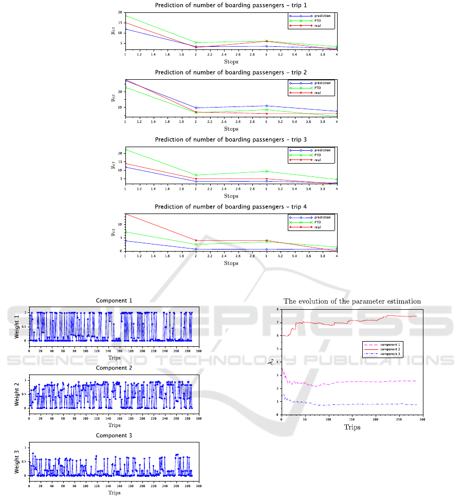
Figure 2: The comparison of predictions, PTD and real values of boarding passengers at four stops and selected trips.
Figure 3: The weight evolution for all trips during the day.
Most current models consider ideal traffic condi-
tions (no delays), e.g. (Roos et al., 2016) or do not in-
clude information about lines at all, e.g. (Lijuan and
Chen, 2017), etc. However, in tram networks, traf-
fic conditions significantly affect passenger demand
for a specific trip. For example, if a tram is delayed,
more passengers use it, because apart from its base
passengers it carries passengers who were supposed
to board the next tram. On the other hand, when arriv-
ing shortly after the previous tram, less passengers use
Figure 4: The parameter estimate evolution at a chosen stop.
it. In complex networks with more lines sharing the
same tracks, there are other variables which affect the
passenger demand on a specific trip (e.g., line rout-
ing). Therefore, incorporating traffic variables mea-
sured in real time can be vital in improving the accu-
racy of the passenger demand model.
ACKNOWLEDGEMENTS
This work has been supported by the project
SILENSE, project number ECSEL 737487 and
MSMT 8A17006.
Modeling of Passenger Demand using Mixture of Poisson Components
623

REFERENCES
Y. Sun, B. Leng and W. Guan, 2015. A novel wavelet-SVM
short-time passenger flow prediction in Beijing sub-
way system. Neurocomputing. 166, 109-121
J.D. Ort
´
uzar and L.G. Willumsen, 1996. Modelling Trans-
port, 2nd Edition. Wiley.
Y. Jia, P. He, S. Liu and L. Cao, 2016. A combined fore-
casting model for passenger flow based on GM and
ARMA. International Journal of Hybrid Information
Technology. 9/2, p. 215–226.
Y. Bai, Z. Sun, B. Zeng, J. Deng and C. Li, 2017. A multi-
pattern deep fusion model for short-term bus passen-
ger flow forecasting. Applied Soft Computing. 58, p.
669–680.
S. Zhao, T. Ni, Y. Wang and X. Gao, 2011 A new approach
to the prediction of passenger flow in a transit system.
Computers and Mathematics with Applications. 61, p.
1968–1974.
L. Liu and R. Chen., 2017. A novel passenger flow predic-
tion model using deep learning methods. Transporta-
tion Research Part C. 84, p. 74–91.
J. Roos, G. Gavin and S. Bonnevay, 2016. A dynamic
Bayesian network approach to forecast short-term ur-
ban rail passenger flows with incomplete data. Trans-
portation Research Procedia. 26, p. 53–61.
S. Haar and S. Theissing, 2015. A hybrid-dynamic model
for passenger-flow in transportation systems. IFAC-
PapersOnLine. 48-27, p. 236–241.
L. Sun, Y. Lu, J. Jin, D. Lee and K. Axhausen, 2015. An
integrated Bayesian approach for passenger flow as-
signment in metro networks. Transportation Research
Part C. 52, p. 116–131.
Y. Li, X. Wang, S. Sun, X. Ma and G. Lu, 2017. Forecast-
ing short-term subway passenger flow under special
events scenarios using multiscale radial basis function
networks. Transportation Research Part C. 77, p. 306–
328.
Z. Ma, J. Xing, M. Mesbad and L. Ferreira, 2014. Predict-
ing short-term bus passenger demand using a pattern
hybrid approach. Transportation Research Part C. 39,
p. 148–163.
M. Milenkovi
ˇ
c, L.
ˇ
Svadlenka, V. Melichar, N. Bojovi
ˇ
c
and Z. Avramovi
ˇ
c., 2016. SARIMA modelling ap-
proach for railway passenger flow forecasting. Trans-
port. 2016, p. 1–8.
C. Zhou, P. Dai and R. Li., 2013. The passenger demand
prediction model on bus networks. In: Proceedings of
13th International Conference on Data Mining Work-
shops. p. 1069-1076.
M. Chen and Y. Wei., 2011. Exploring time variants for
short-term passenger flow. Journal of Transport Ge-
ography. 19, p. 488-498.
T. Tsai, C. Lee and C. Wei, 2009. Neural network based
temporal feature models for short-term railway pas-
senger demand forecasting. Expert Systems with Ap-
plications. 36, p. 3728–3736.
X. Jiang, L. Zhang and X. Chen, 2014. Short-term fore-
casting of high-speed rail demand: A hybrid approach
combining ensemble empirical mode decomposition
and gray support vector machine with real-world ap-
plications in China. Transportation Research Part C.
44, p. 110–127.
S. Haar and S. Theissing, 2016. Forecasting passenger loads
in transportation networks. Electronic Notes in Theo-
retical Computer Science. 327, p. 49–69.
V. Peterka. Bayesian system identification, 1981. In: Trends
and Progress in System Identification, P. Eykhoff, Ed.
Oxford: Pergamon Press, p. 239–304.
M. K
´
arn
´
y, J. Kadlec, E.L. Sutanto, 1998. Quasi-Bayes es-
timation applied to normal mixture. Preprints of the
3rd European IEEE Workshop on Computer-Intensive
Methods in Control and Data Processing, Eds: J.
Roj
´
ı
ˇ
cek, M. Vale
ˇ
ckov
´
a, M. K
´
arn
´
y, K. Warwick, p. 77–
82, CMP ’98 /3./, Prague, CZ, 07.09.1998–09.09.
M. K
´
arn
´
y, J. B
¨
ohm, T. V. Guy, L. Jirsa, I. Nagy, P. Nedoma,
and L. Tesa
ˇ
r, 2006. Optimized Bayesian Dynamic Ad-
vising: Theory and Algorithms. Springer, London.
I. Nagy, E. Suzdaleva, 2017. Algorithms and Programs
of Dynamic Mixture Estimation. Unified Approach
to Different Types of Components, SpringerBriefs in
Statistics. Springer International Publishing, 2017.
P. Samaras, A. Fachantidis and G. Tsoumakas, 2015. A pre-
diction model of passenger demand using AVL and
APC Data from a bus fleet. 19th Panhellenic Confer-
ence on Informatics. p. 129–134.
I. Nagy, E. Suzdaleva, M. K
´
arn
´
y and T. Mlyn
´
a
ˇ
rov
´
a, 2011.
Bayesian estimation of dynamic finite mixtures. Int.
Journal of Adaptive Control and Signal Processing.
25(9), p. 765–787.
S. Yang and G. Berdine, 2015. Poisson regression. The
Southwest Respiratory and Critical Care Chronicles.
3(9), 2015, p. 61–64.
I. Nagy, E. Suzdaleva, P. Pecherkov
´
a, 2016. Comparison
of Various Definitions of Proximity in Mixture Esti-
mation. Proceedings of the 13th International Con-
ference on Informatics in Control, Automation and
Robotics (ICINCO). Lisbon, Portugal, July, 29 – 31,
p. 527–534.
Pu
ˇ
sman V., 2013. Optimalizace syst
´
emu organizace ve
ˇ
rejn
´
e
hromadn
´
e dopravy. The dissertation thesis.
ICINCO 2019 - 16th International Conference on Informatics in Control, Automation and Robotics
624
