Mapping Land Cover Types using Sentinel-2 Imagery: A Case Study

Laura Annovazzi-Lodi, Marica Franzini and Vittorio Casella

Department of Civil Engineering and Architecture, University of Pavia, Via Ferrata 5, Pavia, Italy

Keywords: Sentinel-2, Remote Sensing, Supervised Classification, SVM and Land Cover.

Abstract: This paper presents a case study of automatic classification of the remotely sensed Sentinel-2 imagery, from

the EU Copernicus program. The work involved a study site, located in the area next to the city of Pavia, Italy,

including fields cultivated by three farms. The aim of this work was to evaluate the so-called supervised

classification applied to satellite images and performed with Esri's ArcGIS Pro software and Machine Learn-

ing techniques. The classification performed produces a land use map that is able to discriminate between

different land cover types. By applying the Support Vector Machine (SVM) algorithm, it was found that, in

our case, the pixel-based method offers a better overall performance than the object-based, unless a specific

class is exclusively taken into consideration. This activity represents the first step of a project that fits into the

context of Precision Agriculture, a recent and rapidly developing research area, whose aim is to optimize

traditional cultivation methods.

1 INTRODUCTION

The World Population Prospect document of the

United Nations (DESA, 2017) predicts that the world

population will rise to 9.8 billion by 2050. All over

the planet, there will be a corresponding increment in

food demand, and this is one of the major humanity

challenges.

Furthermore, climate change, environmental deg-

radation, the ever increasing demand for water and

energy, socio-political and economic changes are just

a few examples of factors that necessarily motivate us

to integrate technological innovation in the produc-

tive processes of modern agriculture in a consolidated

way that makes it more fruitful and, at the same time,

sustainable (MiPAAF, 2017), (Chhetri et al., 2012).

Thematic maps show the spatial distribution of a

generic indicator and depict environmental and phys-

ical factors (geological maps, distribution of water re-

sources, entity of precipitations, etc.), biological (dis-

tribution of forests, surface of agricultural crops and

their production, etc.) or social ones (census distribu-

tion, population’s average age, health, etc.). Land use

maps are particular thematic maps where the terrain

is subdivided into several categories belonging to a

pre-defined list such as: roads, buildings, forest, fields

and so on: the level of detail of the classification de-

pends on the goal and on the degree of detail of the

data used to produce the map.

The most used way to produce large-scale land

use maps is the classification of remote sensing im-

ages.

Among land cover maps, crop type maps are nec-

essary for different purposes and provide crucial in-

formation for monitoring and management of the ag-

ricultural sector. According to (Marais-Sicre et al.,

2016) they can be employed, for example, to estimate

the specific use of water for a certain type of cultiva-

tion or to identify the various types of crops before

the start of the irrigation season, so as to study the best

strategy resource management for water, which is

both sustainable and resourceful. They are also useful

in creating growth models that allow for estimation of

crop yield.

These maps are therefore essential in the field of

Precision Agriculture (PA). PA is the application of

technologies and principles to manage spatial and

temporal variability associated with all aspects of ag-

ricultural production for improving crop performance

and environmental quality (Pierce and Nowak, 1999).

PA is based on a bunch of Geomatics techniques: ter-

ritory survey, satellite navigation and GIS. Crop maps

are also required by policy and decision-makers for

economics, management and for agricultural statistics

(Immitzer et al., 2016). Information recorded and pro-

duced in the frame of PA could facilitate different ad-

ministrative and control procedures (Zarco-Tejada et

al., 2014).

242

Annovazzi-Lodi, L., Franzini, M. and Casella, V.

Mapping Land Cover Types using Sentinel-2 Imagery: A Case Study.

DOI: 10.5220/0007738902420249

In Proceedings of the 5th International Conference on Geographical Information Systems Theory, Applications and Management (GISTAM 2019), pages 242-249

ISBN: 978-989-758-371-1

The goal of this study is to assess supervised clas-

sification, both object- and pixel-based, applied to a

Sentinel-2 image. This activity is the first step of a

project of classification of parcels of land according

to the type of agricultural crop practiced, that fits into

the context of PA.

2 MATERIALS

2.1 Study Area

The study site (Figure 1) is located about 15 km north-

west of the city of Pavia, Italy; it covers a total area

of 3220 ha. The considered site belongs to the terri-

tory of the Pianura Padana, which offers the best con-

ditions for the cultivation of rice: wet climate, loose

soil and large water availability. The study area con-

tains different land covers/use categories such as

cropland, woods, industrial and urban areas, roads

and a stretch of the river Ticino including its mean-

ders.

2.2 Ground Truth

By interviewing farm owners, in situ reference data

concerning the year 2017, was collected. The infor-

mation gathered for each agricultural plot was crop

type, sowing and harvesting date. The plots are char-

acterized by a large variety of shapes (square, rectan-

gular or triangular). The main cultivated crops in this

region are ryegrass, maize, barley, grassland, rice, rye

and soybean.

The reference data concerning the rest of the site,

such as the water of the river Ticino or the asphalt of

the roads, was obtained observing a very high-resolu-

tion satellite image, acquired by Digital Globe and

provided by Esri within its products; its ground reso-

lution is, for the considered area, 30 cm. The so-ob-

tained data was also verified both by examining the

relative Google Street View images and by direct in-

spection of the areas under study.

Based on the data collected and observed, 439

polygons were manually drawn and created, corre-

sponding to a total area of just over 800 ha. To pre-

cisely draw the polygons, the raster maps of the fun-

damental regional cartography were downloaded

from the Geoportal of the Lombardy Region (URL-

1), related to the area of interest. Since the regional

maps are not completely up-to-date, and are therefore

considered only partially reliable, the high-resolution

satellite image mentioned above was jointly used as

base map.

It was decided to eliminate polygons exclusively

dedicated to rye, soybean, pea and other vegetables

(and not the plots intended for catch crop cultivation)

because the number of polygons was not sufficient to

create a distinction of the spectral signature, as well

as to avoid large class imbalances. Hence, the final

number of polygons taken into consideration for our

study was 418, with a total area of almost 774 ha (Ta-

ble 1).

The so-obtained ground truth map is organized as

a time-dependent GIS layer. The record associated

with each polygon has a textual field describing the

time frame of the various crops related to it. Once a

date is chosen, a truth map containing the real classi-

fication at that time can be defined by manually filling

a numeric field.

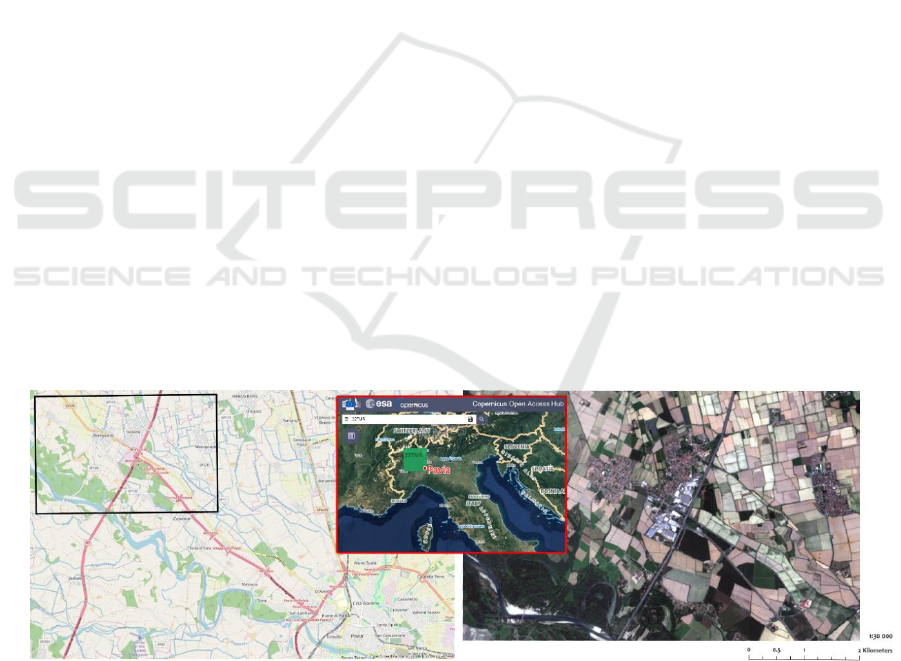
Figure 1: On the left: the study area (framed in black), next to the city of Pavia [Open Street Map]. In the middle: the extent

of the Sentinel-2 Tile 32TMR (https://scihub.copernicus.eu/dhus/#/home). On the right: S-2 scene (TCI) of the study area.

Mapping Land Cover Types using Sentinel-2 Imagery: A Case Study

243

Table 1: Number of polygons and surface corresponding to

each class.

Class

Number of

polygons

(ha)

Water

16.47

Asphalt

8.92

Wood

111.63

Industrial

15.85

Barley

39.12

Grassland

85.44

Bare soil

199

427.56

Urban

68.48

TOT.

418

773.47

2.3 Satellite Data and Crop Phenology

Sentinel-2 mission is a land monitoring constellation

of two satellites (Sentinel-2A and Sentinel-2B, re-

spectively launched on 22.06.2015 and on 7.03.2017)

flying in the same orbit but phased at 180°, designed

to give a high revisit frequency of 5 days at the Equa-

tor. It carries an innovative wide-swath, high-resolu-

tion, multi-spectral imager (MSI) with 13 spectral

bands with 10, 20 and 60 m spatial resolution.

In this study, since the data collected was relative

to the year 2017, all the S-2 images of that year were

downloaded (concerning the area of interest, corre-

sponding to the tile 32TMR - ESA’s scene naming

convention). After visual inspection, it was decided to

exclude the images with high cloud coverage at the

granule level and with cloud cover concentrated right

in the study area. Therefore, 15 images (out of 109)

were taken into consideration. Eventually, the image

acquired on May 17 was chosen. The choice was con-

sidered optimal for our classification and was defined

after careful considerations of several aspects listed

below.

For the differentiation of crop types, phenology is

considered as a key factor.

Phenology is defined as the periodicity of key

events in the life cycle of living species, their chro-

nology and their relationship between climate factors

and seasonal events over time (Schwartz, 2003). For

this reason, a chronogram was created, ranging from

March to November and related to the major crop

types (Figure 2).

During the interviews, it was possible to collect

information on the timing of the vegetation cycles and

the phenology of the agricultural crops that are pre-

sent in the study area. The so-obtained knowledge

base has been further implemented by materials found

on the internet and on common agricultural books.

Ryegrass is an autumn-winter forage crop that

grows rapidly. It is sown from the end of September

to the beginning of November, while the harvest usu-

ally takes place in April. This plant is suitable for ro-

tation with maize, with which it is replaced from May

until mid-June.

Maize is one of the most important and wide-

spread cereal crops in our country. Since it requires a

warm and temperate climate, to facilitate its growth

at ever-mild temperatures, sowing usually takes place

from the end of March to April-May, but may con-

tinue until mid-June. The emergency phase can occur

up to about 20 days later. Harvest takes place from

the beginning of August to October.

Grassland is a stable lawn whose phenology de-

pends on certain factors such as climatic conditions,

type of soil and use (hayfields, grazed grassland or

water meadow).

The water meadow is a land permanently irrigated

in winter months by a veil of water, which flows by

gravity in order to prevent the excessive cooling of

the ground. Such a technique allows the grass to grow

even at low temperatures. The water is kept moving

by the slight slope of the ground. During the summer

season, however, periodic irrigations of the area are

carried out, as in a common lawn. In the area of the

river Ticino, given the particular conformation of

humps and valleys typical of these dedicated fields,

the cultivation of water meadows is difficult, but for

its historical importance, about 300 hectares have

been preserved.

Figure 2: Chronogram of sowing and harvesting periods of crops belonging to the largest number of polygons.

Phase

1|15 16|31 1|15 16|30 1|15 16|31 1|15 16|30 1|15 16|31 1|15 16|31 1|15 16|30 1|15 16|31 1|15 16|30

Sowing Ryegrass Ryegrass

Mai ze Mai ze

Barley Barley

Rice

Soybean

Harvest

Barley Barley

Rice

March

April

May

June

November

Ryegrass

September

October

Mai ze

July

August

Soybean

Ryegrass

Mai ze

Rice

Soybean

Mai ze

Rice

Mai ze

GISTAM 2019 - 5th International Conference on Geographical Information Systems Theory, Applications and Management

244

Barley is an unripe crop and the calendar of its

vegetation cycle is rather short, giving it an excellent

adaptability to very different environments. The vari-

eties used in the study area have a good resistance to

cold, so barley is sown between the end of October

and early November. The harvesting phase takes

place at the beginning of summer. Coming to rice, its

sowing season is from April to May. In September,

when the plant has reached full ripeness, the harvest

begins, which lasts until October.

Based on the reported considerations, the autumn-

winter dates have been excluded because almost all

polygons belong to the "bare soil" category, leading

to poorly significant results. May 17

was chosen be-

cause the existing crops are well defined. Indeed,

mid-May is the sowing period of maize and rice

crops, so their related plots are still identifiable as

“bare soil”. Barley, on the other hand, is ready to be

harvested, so well developed and distinguishable.

Even grassland, sown in April, is lush and flourishing.

In conclusion, eight categories were considered

for the described classification experiment. They are

listed in Table 1 and include as agricultural crops:

barley, permanent grass and wood. Also, the ground

truth map was defined according to the general sched-

ule described by the farmers; but real activities

(shown in the image) can be slightly misaligned,

therefore the map was tuned by observing the selected

Sentinel-2 image; the adopted map is shown in Fig. 3.

3 METHODS

Different processes were applied to the collected data,

by using the ESRI ArcGIS Pro software program, in

order to create the land cover map. The workflow is

summarized below (Figure 4):

Figure 4: Workflow of our study.

Figure 3: Ground Truth corresponding to 17 May 2017. The background image is the S-2 scene (TCI) of the study area.

Mapping Land Cover Types using Sentinel-2 Imagery: A Case Study

245

3.1 Pre-processing

Firstly, it should be noted that each S-2 tile covers an

area of 100 km x 100 km. With the aim to alleviate

the load of data during the processing stages of clas-

sification, the tile was clipped in order to circum-

scribe only the area of interest for our study. Atmos-

pheric correction was not necessary because the im-

age was clear within the study site: cloud-free Level

1 image (ToA reflectance) was used. Thanks to the

flat terrain and the good geolocation accuracy, geo-

metric pre-processing was not needed either.

For this study, it was decided to exclude the three

atmospheric bands at 60 m, i.e. B1 Coastal Aerosol,

B9 Water Vapor and B10 SWIR Cirrus. The four

spectral bands B2 Blue, B3 Green, B4 Red and B8

NIR have a resolution of 10 m. The remaining six

bands acquired at 20 m, i.e. the three of Red Edge

such as B5, B6 and B7 and B8A Narrow NIR, and the

two of SWIR such as B11 and B12, have been

resampled. This was done in order to obtain a layer

stack of 10 spectral bands at 10 m. After being

resampled, each band layer has been equalized. In-

deed, pixel values in each band layer were linearly

stretched to the [0, 65535] interval, to give each layer

the same weight, being classification sensitive to the

range of gray levels.

The next step in the workflow was to apply the

Principal Component Analysis (PCA). This is a math-

ematical method used in multivariate statistics to con-

vert a set of variables that are probably correlated to

a set of independent variables, called principal com-

ponents, by using a linear transformation (Abdi and

Williams, 2010). All the principal components are

linear combinations of the original variables and are

orthogonal to each other and therefore independent.

The newly-generated components are sorted so that

most of the information is mainly concentrated in the

first few bands. In our case, the first three compo-

nents, containing more than 99% of the original infor-

mation, were only kept. It should also be noted that

the first component itself contains 95% (Table 2).

Table 2: Results of the PCA step.

PERCENT AND ACCUMULATIVE EIGENVALUES

Layer

Eigen Value

Percent of

Eigen Values

Accumulative of

Eigen Values

15545565733,63619

95,1596

431399292,54862

2,6407

97,8003

300945980,90906

1,8422

99,6425

48264348,94573

0,2954

99,9379

4919188,92151

0,0301

99,9680

2071351,24574

0,0127

99,9807

1343666,65108

0,0082

99,9889

1082935,84931

0,0066

99,9956

425339,96901

0,0026

99,9982

297827,18188

0,0018

100,0000

In the present work, pixel-based classification is

tackled, as well as object-based. The latter implies

that image is segmented: adjacent pixels with similar

spectral bands are grouped. Then segments are treated

as a whole and classified.

ArcGIS adopts the mean shift algorithm that is a

non-parametric, feature-space analysis technique for

locating the maxima of a density function (Fukunaga

and Hostetler, 1975), (Comaniciu and Meer, 2002).

The software requires three parameters: spectral de-

tail, spatial detail and minimum segment size. The

first one sets the level of importance given to spectral

differences between pixels. The second parameter

controls the level of relevance given to the proximity

between pixels. The last one represents a merging cri-

terion. It is good practice to test different combina-

tions of the parameters until the desired result is

found.

Based on our experience and after visually evalu-

ating the result of segmentation, the final parameters

chosen are shown in Table 3.

Table 3: Parameters sets for the segmentation.

Spectral

detail

Spatial

detail

Minimum segment

size in pixels

3.2 Classification

In general, the main objective of supervised tech-

niques (adopted in the present work) is to learn from

a training data set and to be able to make predictions,

i.e. give unclassified pixels or segment a label.

Ground Truth datasets are typically split into two dis-

tinct group and intended for two different functions:

-Training samples: once selected and labeled,

they are used to train the algorithm and to generate

a classification scheme, based on spectral signa-

tures to be applied to the rest of the objects/ pixels

with unknown labels;

-Test set (or Reference dataset): such samples are

not used for training and, being labelled, can be

used to assess the accuracy of classification, in a

statistically independent and rigorous way.

Indeed, a supervised classification consists of

three phases. The first (learning or calibration phase)

and the second (prediction phase) employ training

samples, instead the last one (validation phase) uses

test sets. We used 50% of Ground Truth for training

and 50% for validation.

A number of algorithms for supervised classifica-

tion have been developed over time. We selected the

multiclass Support Vector Machine (SVM) because it

provides a powerful, robust and modern method. The

GISTAM 2019 - 5th International Conference on Geographical Information Systems Theory, Applications and Management

246

principal advantage of this machine-learning algo-

rithm is that it can successfully work with a small

number of training samples (Taskin et al., 2011), as

in our case. Developed by Vapnik and his collabora-

tors, instead of estimating the probability densities of

the classes, it directly solves the problem of interest

by determining the classification boundaries between

the classes (Vapnik, 1979). Basically, the algorithm

tries to find optimal hyperplanes to separate training

samples into a predefined number of classes and by

maximizing the margin between the classes, looking

for hyperplanes as distant as possible from the train-

ing samples of classes (Kowalczyk, 2017). It is also

able to separate non-linear problems through the so-

called SVM trick, based on the kernel method.

3.3 Accuracy Assessment

Without a validation phase, the final classified map

cannot be reliably used and, therefore, its applicabil-

ity is limited. The accuracy of the classified image is

assessed by comparing the classified map, obtained

from the classification process, with the reference da-

taset. It should be noted that, usually, validation does

not occur by verifying all the pixels contained in the

test set, but only a limited number. We decided to ran-

domly generate 5000 points from the test set of poly-

gons and compare the prediction and ground truth

with them. The validation phase provides information

on the product quality and identifies probable sources

of error by analyzing the confusion matrix, which

summarizes the correct and incorrect predictions

made. For pixel- and object-based classifications, the

information contained in the confusion matrix is used

to evaluate some common statistical measures, which

express the quality of the classification. These in-

cluded the overall accuracy (OA), the producer’s ac-

curacy (PA), the user’s accuracy (UA), the omission

and the commission errors, and the Kappa coefficient.

4 RESULTS AND DISCUSSION

In this section, classification results and accuracy as-

sessment are shown. As already introduced, we per-

formed both object- and pixel-based classification us-

ing the SVM algorithm. Three iterations were per-

formed: the first one with the 8 classes listed in Tab.1;

the second iteration with 7 classes as Asphalt and Ur-

ban were merged; the third one with 6 classes as In-

dustrial was merged too. Tables 4 to 7 show the con-

fusion matrix for object- and pixel-based classifica-

tion, for iteration 1 and 2; the third iteration is not il-

lustrated since it gave limited improvements.

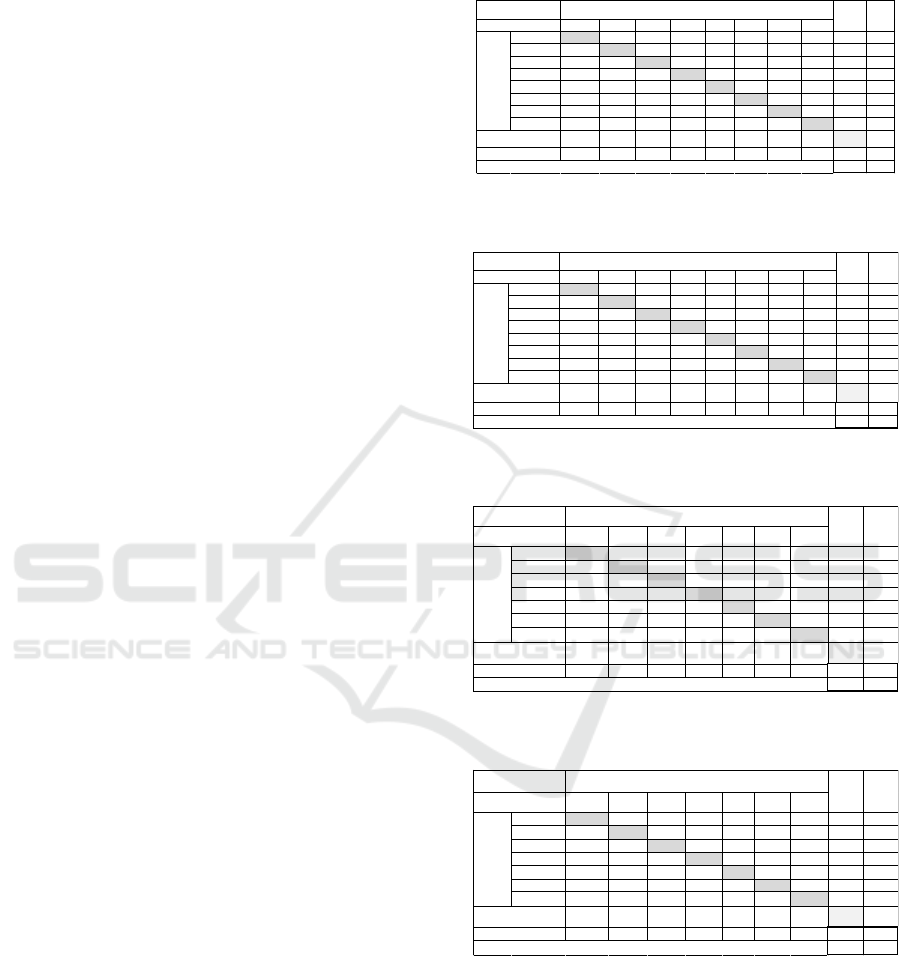
Table 4: Confusion matrix for the first object-based classi-

fication.

Table 5: Confusion matrix for the first pixel-based classifi-

cation.

Table 6: Confusion matrix for the second object-based clas-

sification.

Table 7: Confusion matrix for the second pixel-based clas-

sification.

Concerning the first iteration, the two methods

achieved a satisfactory overall accuracy and a very

good Kappa coefficient, presenting minimal differ-

ences. However, by analyzing the confusion matrix in

detail, we observed errors.

In relation to the object-based classification (Ta-

ble 4), the lower PA is that of Asphalt with a value of

26%. The Asphalt class was often confused with that

of the Urban. We did not observe the opposite error,

Bare soil Urban Industrial Asphalt Water Grassland Wood Barley

Bare soil 2552 33 10 13 16 34 2 8 2668 0.957

Urban 250 366 13 20 0 2 0 0 651 0.562

Industrial 1 0 46 0 0 0 0 0 47 0.979

Asphalt 0 0 0 12 0 0 1 0 13 0.923

Water 0 0 0 0 68 0 0 0 68 1.000

Grassland 2 0 0 0 0 430 16 21 469 0.917

Wood 73 0 1 1 0 25 633 36 769 0.823

Barley 21 0 0 0 5 57 64 170 317 0.536

2899 399 70 46 89 548 716 235 5002

0.880 0.917 0.657 0.261 0.764 0.785 0.884 0.723 OA 0.855

Kappa 0.775

Classified

Totals

Reference Totals

Classified Data

Reference Dataset

Object-based

Bare soil Urban Industrial Asphalt Water Grassland Wood Barley

Bare soil 2514 72 26 13 4 29 23 30 2711 0.927

Urban 276 312 6 14 0 4 0 0 612 0.510

Industrial 2 9 38 3 0 0 0 0 52 0.731

Asphalt 4 4 0 15 0 0 1 1 25 0.600

Water 0 0 0 0 85 0 0 0 85 1.000

Grassland 40 1 0 0 0 452 7 38 538 0.840

Wood 25 1 0 0 0 22 640 19 707 0.905

Barley 38 0 0 1 0 41 45 147 272 0.540

2899 399 70 46 89 548 716 235 5002

0.867 0.782 0.543 0.326 0.955 0.825 0.894 0.626 OA 0.840

Kappa 0.751

Classified

Totals

Reference Totals

Reference Dataset

Classified Data

Pixel-based

Bare soil Industrial Water Grassland Wood Barley

Asphalt+

Urban

Bare soil 2538 24 7 27 20 36 97 2749 0.923

Industrial 9 39 0 0 0 0 19 67 0.582

Water 2 0 82 0 0 1 0 85 0.965

Grassland 51 0 0 453 2 28 0 534 0.848

Wood 23 0 0 15 648 22 2 710 0.913

Barley 19 0 0 50 45 148 0 262 0.565

Asphalt+Urban 257 7 0 3 1 0 326 594 0.549

2899 70 89 548 716 235 444 5001

0.875 0.557 0.921 0.827 0.905 0.630 0.734 OA 0.847

Kappa 0.759

Reference Totals

Classified

Totals

Classified Data

Reference Dataset

Pixel-based

Bare soil Industrial Water Grassland Wood Barley

Asphalt+

Urban

Bare soil 2380 2 39 42 21 3 151 2638 0.902

Industrial 8 117 0 0 0 0 19 144 0.813

Water 0 0 70 0 0 0 0 70 1.000

Grassland 5 0 0 462 9 3 0 479 0.965

Wood 43 0 16 35 620 10 3 727 0.853

Barley 40 0 0 16 36 255 1 348 0.733

Asphalt+Urban 151 17 0 1 42 0 383 594 0.645

2627 136 125 556 728 271 557 5000

0.906 0.860 0.560 0.831 0.852 0.941 0.688 OA 0.857

Kappa 0.788

Reference Totals

Classified Data

Reference Dataset

Classified

Totals

Object-based

Mapping Land Cover Types using Sentinel-2 Imagery: A Case Study

247

i.e. Urban was never classified as Asphalt. In addi-

tion, the Industrial class was classified as Urban in 13

cases out of 70, resulting in a PA of 66%. Also, in this

case, the opposite error was never observed, i.e. Ur-

ban was never classified as Industrial. As concerning

the UA, we have low values for the Urban, which was

classified as Bare Soil (250 out of 651), as we can see

in Table 4. Similarly, in the pixel-based confusion

matrix (Table 5), it was possible to observe confusion

between Urban and Asphalt categories (although

slightly less frequent) and classification errors be-

tween Bare soil and Urban classes (a little more fre-

quent). The distinction between Urban, Industrial and

Asphalt classes is not a major requirement in view of

our future project of crop detection. As already men-

tioned, given the described classification errors, it

was decided to perform a second iteration after merg-

ing the Urban and Asphalt classes and a third one by

aggregating Industrial too. Such strategy aimed at im-

proving accuracy without losing discrimination

power between agricultural crops.

A third iteration did not achieve a substantial im-

provement, and therefore results from the second one

(characterized by the merge of Asphalt and Urban

into a unique category) are briefly discussed.

By observing the confusion matrix derived from the

second iteration of the object-based classification

(Table 6), and comparing it with that corresponding

to the first iteration, it was immediately observed that

all the PA values were greater than 0.5 and those of

the UA were greater than 0.6. In particular, for the

Asphalt class the low PA of 0.26 did not appear. The

same observation can be applied to the second itera-

tion of pixel-based classification matrix (Table 7),

compared with the corresponding matrix of the first

iteration. The PA values were always higher than

0.55, whereas the UA was always higher than 0.54. In

particular, for the Asphalt class the low PA of 0.33

did not appear. On the other hand, a reduction of the

PA and UA accuracy of some classes, for example the

PA of Water in the object-based matrix, was found.

Essentially, there were fewer accuracy problems with

the pixel-based classification.

Figure 5: Land cover maps resulting from the first iteration. On the left: Object-based classification. On the right: Pixel-based

classification.

Figure 6: Land cover maps resulting from the second iteration, after merging Asphalt and Urban (seven land cover types). On

the left: Object-based classification. On the right. Pixel-based classification.

GISTAM 2019 - 5th International Conference on Geographical Information Systems Theory, Applications and Management

248

The direct comparison between the two matrices

of the second iteration shows that the object-based

classification is more suitable for the Industrial class

and for the Barley class, while the pixel-based classi-

fication better predicts Water. Naturally, the improve-

ment of both compared to the first level is due pre-

cisely to the incorporation of classes Asphalt and Ur-

ban. It can be said that, in general, the pixel-based

method offers a higher average performance than the

object-based, unless a specific class is only focused.

Table 8: Overall Accuracy Summary of the first and second

iteration.

I object-

based

I pixel-

based

II object-

based

II pixel-

based

0.855

0.840

0.857

0.846

Land cover maps for both methodologies and iter-

ations 1 and 2 are shown in Figures 5, 6.

A final remark concerns processing time. Object-

based classification takes a few minutes for segmen-

tation on a quad-code personal computer and another

few minutes for training and classification. Pixel-

based needs several hours.

5 CONCLUSIONS

The workflow presented in this study was developed

with the aim of evaluating the potentials obtainable

from the classification of remote sensing images pro-

vided by the Sentinel-2 satellites, in particular that of

creating land covers and use maps. The study area

concerned a neighboring area to the town of Pavia,

Italy. Data for training and accuracy assessment was

personally collected by interviewing farm owners,

observing a very high-resolution satellite image and

with inspection of the areas pertained to as well. The

date May 17

2017 was chosen for the study.

As inputs, 10 spectral bands resampled to 10 m

were used. Through ArcGIS Pro (Esri), the pixel-

based and object-based supervised classifications

were applied, using the multiclass SVM algorithm.

The procedures were iterative, to best satisfy the lev-

els of accuracy desired. Thanks to the different bands

available that allow recognizing specific spectral sig-

natures for the objects observed, the multispectral im-

age used has been well suited to the identification of

the different types of coverage present in the area of

interest. It can be said that in general the pixel-based

method offers a better average performance than the

object-based one, unless interested in specific classes.

However, the two methods offer a comparable overall

accuracy. On the other hand, it is also necessary to

take into account the processing time: a few minutes

in the case of object-based classification, several

hours for the pixel-based method. Considering the

overall accuracy results obtained in this study (Table

8), we can conclude that the supervised method is

quite effective for land cover detection.

REFERENCES

Abdi, H., Williams, L. J., 2010. Principal component analy-

sis. In Wiley Interdisciplinary Reviews: Computational

Statistics, vol. 2, no. 4, pp. 433-459.

Chhetri, N., Chaudhary, P., Tiwari, P. R., Yadaw, R. B.,

2012. Institutional and technological innovation: Under-

standing agricultural adaptation to climate change in Ne-

pal. Applied Geography, 33, 142-150.

Comaniciu, D., Meer, P., 2002. Mean shift: A robust ap-

proach toward feature space analysis. IEEE Trans. Pat-

tern Anal. Mach. Intell. , 24, 603–619.

DESA, U., 2017. World population prospects, the 2017 Re-

vision, Volume I: comprehensive tables. New York

United Nations Department of Economic & Social Af-

fairs.

Fukunaga, K., Hostetler, L., 1975. The estimation of the gra-

dient of a density function, with applications in pattern

recognition. IEEE Trans. Inf. Theory, 21, 32–40.

Immitzer, M., Vuolo, F., Atzberger, C., 2016. First Experi-

ence with Sentinel-2 Data for Crop and Tree Species

Classiﬁcations in Central Europe, Remote Sensing.

Kowalczyk, A., 2017. Support Vector Machines succinctly,

Succinctly E-book series, Syncfusion Inc.

Marais-Sicre, C., Inglada, J., Fieuzal, R., Baup, F., Valero, S.,

Cros, J., Huc, M., Demarez, V., 2016. Early Detection of

Summer Crops Using High Spatial Resolution Optical

Image Time Series, Remote Sensing.

MiPAAF, 2017. Linee Guida per lo Sviluppo

dell’Agricoltura di precisione in Italia. In Pubblicazioni

Ministero delle Politiche Agricole Alimentari e Forestali

Pierce, F. J., Nowak, P., 1999. Aspects of precision agricul-

ture. In Advances in agronomy.

Schwartz, M. D., 2003. Phenology: An Integrative Environ-

mental Science, Dordrecht: Kluwer Academic Publish-

ers.

Taskin Kaya, G., Musaoglu, N., Ersoy, O. K., 2011. Damage

assessment of 2010 Haiti earthquake with post-earth-

quake satellite image by support vector selection and ad-

aptation. Photogrammetric Engineering & Remote Sens-

ing, 77(10), 1025-1035.

URL-1: http://www.geoportale.regione.lombardia.it

Vapnik, V., 1979. Estimation of Dependences Based on Em-

pirical Data. Nauka, Moscow, pp. 5165–5184, 27 (in

Russian) (English translation: Springer Verlag, New

York, 1982).

Zarco-Tejada, P., Hubbard, N., Loudjani, P., 2014. Precision

Agriculture: An Opportunity for EU Farmers - Potential

Support with the CAP 2014-2020. In Joint Research

Centre (JRC) of the European Commission publication

Mapping Land Cover Types using Sentinel-2 Imagery: A Case Study

249