
Performance Prediction of GPU-based Deep Learning Applications
Eugenio Gianniti
1
, Li Zhang
2
and Danilo Ardagna
1
1
Dip. Elettronica, Informazione e Bioingegneria, Politecnico di Milano, Milan, Italy
2
IBM Research, Yorktown Heights, N.Y., U.S.A.
Keywords:
Convolutional Neural Networks, Deep Learning, Performance Prediction, General Purpose GPUs.
Abstract:
Recent years saw an increasing success in the application of deep learning methods across various domains
and for tackling different problems, ranging from image recognition and classification to text processing and
speech recognition. In this paper we propose, discuss, and validate a black box approach to model the execu-
tion time for training convolutional neural networks (CNNs), with a particular focus on deployments on general
purpose graphics processing units (GPGPUs). We demonstrate that our approach is generally applicable to a
variety of CNN models and different types of GPGPUs with high accuracy. The proposed method can support
with great precision (within 5% average percentage error) the management of production environments.
1 INTRODUCTION
Nowadays, convolutional neural networks (CNNs)
find application across industries, most notably for
image recognition and classification tasks, which rep-
resented the first successful adoption of the tech-
nique (Krizhevsky et al., 2012). Ranging from med-
ical diagnosis to public security, deep learning (DL)
methods are fruitfully exploited in a wide gamut of
products. In addition to the established applications,
there is ongoing work on the technique’s adaptation
for other use cases, like speech recognition (Sainath
et al., 2015) and machine translation (Bahdanau et al.,
2014).
CNNs hail from regular neural networks (NNs),
but improve on them by reducing the connectivity pat-
tern and by introducing novel layers specifically de-
signed to take advantage of the peculiarities shown by
images (Krizhevsky et al., 2012). The common archi-
tecture for basic NNs is composed of a number of neu-
ron layers organized so that subsequent ones are com-
pletely connected, but without any link among same-
layer neurons or bypassing connections (Srivastava
et al., 2014). This design is well suited for datasets
with a limited set of features that simply become the
input for the first neuron layer, but colored images can
easily provide one million of values if their raw pixels
are to be fed as data into the network, even at very low
resolution: NNs at such a scale are computationally
impractical. In order to work around the issue, CNNs
introduce a series of new layer typologies, in partic-
ular the namesake convolutional one (Szegedy et al.,
2015). The general idea is to devise sparser connec-
tivity patterns, so as to reduce the computational com-
plexity and render the problem tractable, but at the
same time to stack several layers, in order to incre-
mentally achieve the same global view of the feature
space offered by ordinary fully connected ones.
Over time, many frameworks have been devel-
oped to provide high level APIs for CNN design,
learning, and deployment. Among the most well
known, we recall Torch, PyTorch, TensorFlow, and
Caffe. Usually DL models are trained by relying on
GPGPU systems (even in clusters for experimental
environments (Wang et al., 2017)), which allow to
achieve from 5 up to 40x time improvement when
compared to CPU deployments (Bahrampour et al.,
2015).
In spite of the widespread adoption of DL sys-
tems, still there are few studies taking a system per-
spective which aim at investigating how, e.g., the
training time changes when running on different
GPGPUs or by varying the number of training itera-
tions or the batch size (Bahrampour et al., 2015; Had-
jis et al., 2016). DL applications are characterized
by a large number of design choices that often do not
apply readily to other domains or hardware configu-
rations, up to the point that even advanced users with
considerable DL expertise fail at identifying optimal
configuration settings (Hadjis et al., 2016).
The time required to train a new DL model is gen-
erally unknown in advance. Because of this, perfor-
Gianniti, E., Zhang, L. and Ardagna, D.
Performance Prediction of GPU-based Deep Learning Applications.
DOI: 10.5220/0007681802790286
In Proceedings of the 9th International Conference on Cloud Computing and Services Science (CLOSER 2019), pages 279-286
ISBN: 978-989-758-365-0
Copyright
c
2019 by SCITEPRESS – Science and Technology Publications, Lda. All rights reserved
279

mance analysis is usually done empirically through
experimentation, requiring a costly setup (Bahram-
pour et al., 2015). Performance modeling can help,
e.g., to establish service level agreements with end
users or to predict the budget to train or run produc-
tion DL models in the cloud.
In this paper, we present a method to learn perfor-
mance models for CNNs running on a single GPGPU.
The main metrics under investigation are the forward
time, relevant to quantify the time taken for classifi-
cation when the trained network is deployed, and the
gradient computation time, which on the other hand
is important during the learning phase. In the follow-
ing, we will generally mention forward and backward
passes, referring to the direction in which information
flows through the CNN, with either features incre-
mentally processed for classification or partial deriva-
tives that back propagate to reach learnable weights.
Our goal is to lead new users with limited previ-
ous experience from an initial test deployment to real
scale applications. In order to meet the requirements
of both scenarios, i.e., the generality needed in the
preliminary design phase of a project on one side and
the high accuracy expected when running in produc-
tion on the other, we envision two alternative tech-
niques to derive models that boast different trade-offs.
In our previous work (Gianniti et al., 2018), we
proposed a gray box per layer approach where model-
ing is performed layer by layer and the only explana-
tory variable is computational complexity. This tech-
nique allows for great generality, since partial layer
predictions can be easily combined into a full CNN
estimate, even if the specific network schema has
never been considered as part of the training set. Due
to this, the approach is preeminently interesting dur-
ing the initial design stages, for instance to compare
different alternative CNNs and deployments in terms
of performance. On the other hand, when a deploy-
ment is already available, data coming from the real
system enables a different approach with its focus on
precision rather than ease of generalization.
This second scenario can be tackled with a black
box approach, called end to end modeling, which fo-
cuses on a single CNN and learns the dependency of
execution time on varying batch size and iterations
number. The improved accuracy comes at the expense
of a quite narrower focus centered around a particu-
lar network architecture and deployment, which pre-
vents the application of the model in different situa-
tions. Moreover, this modeling technique requires a
collection of historical data, thus entailing either an
experimental campaign or the proper monitoring of
previous runs in a production environment. However,
as we will demonstrate through our empirical analy-
ses, small scale experiments are enough to extrapolate
to a larger scale range, which mitigates the cost of this
approach.
In our experimental campaign, we considered
three popular DL models, implemented with the Caffe
framework and run on two different GPGPUs. Yet our
methodology is not constrained in any way neither to
a specific framework, nor GPGPU model. The out-
comes show that we can either obtain per layer mod-
els general enough to yield relative errors below 10%
on average across different CNN architectures and be-
low 23% in the worst case, or more specialized on a
specific end to end scheme, but accurate within 5% of
measured execution times.
Our contributions in this paper are as follows: 1)
an end to end model capable of predicting both learn-
ing and inference of a convolutional network in a pro-
duction environment, 2) a comparison of the end to
end with the per layer model proposed in (Gianniti
et al., 2018).
This paper is organized as follows. An overview
of other literature proposals is provided in Section 2,
while Section 3 introduces the end to end, black box
performance model. Its accuracy and a discussion of
the key findings of our experimental analysis are re-
ported in Section 4. Conclusions are finally drawn in
Section 5.
2 RELATED WORK
DL popularity is steadily increasing thanks to its im-
pact on many application domains (ranging from im-
age and voice recognition to text processing) and
has received a lot of interest from many academic
and industry groups. Advances are boosted by en-
hancements of the deep networks structure and learn-
ing process (e.g., dropout (Srivastava et al., 2014),
network in network (Lin et al., 2013), scale jitter-
ing (Vincent et al., 2010)) and by the availability of
GPUs, which allows to gain up to 40x improvement
over CPU systems (Bahrampour et al., 2015).
Over the last few years, several frameworks have
been developed and are constantly extended to ease
the development of DL models and to optimize dif-
ferent aspects of training and deployment of DL ap-
plications. The work in (Bahrampour et al., 2015)
provides a comparative study of Caffe, Neon, Theano,
and Torch, by analyzing their extensibility and perfor-
mance and considering both CPUs and GPUs. The
paper provides insights on how performance varies
across batch sizes and different convolution algorithm
implementations, but it does not provide means to
generalize performance estimates.
CLOSER 2019 - 9th International Conference on Cloud Computing and Services Science
280

The authors of (Jia et al., 2012) propose the
Stargazer framework to build performance models
for a simulator running on GPU, so as to correlate
several GPU parameters to the simulator execution
time. Given the daunting size of the design space,
which considers very low level parameters, they ex-
ploit sparse random sampling and iterative model se-
lection, thus creating step by step an accurate lin-
ear regression model. Another approach is proposed
in (Liu et al., 2007), where the authors elaborate a
detailed analytical model of general purpose appli-
cations on GPUs, consisting of three general expres-
sions to estimate the time taken for common opera-
tions, according to their dependencies on data size or
computational capabilities. Similar analytical model-
ing approaches (Baghsorkhi et al., 2010; Zhang and
Owens, 2011; Hong and Kim, 2009; Song et al.,
2013) rely on micro-architecture information to pre-
dict GPU performance. As GPU architectures con-
tinue to evolve, the main issue of analytical models is
that any minor change may require extensive work for
adapting models.
Given the complexity of GPU hardware (many
cores, context switching, memory subsystem, etc.),
recently black box approaches based on machine
learning (ML) are favored over analytical models. In-
deed, black box techniques allow for deriving per-
formance models from data and making predictions
without a priori knowledge about the internals of the
target system. On the other hand, ML models (Dao
et al., 2015; Barnes et al., 2008; Bitirgen et al., 2008;
Kerr et al., 2010; Lu et al., 2017; Gupta et al., 2018)
require to perform an initial profiling campaign to
gather training data. An overview and quantitative
comparison among recent analytical and ML-based
model proposals is reported in (Madougou et al.,
2016).
In this research area, the authors of (Venkataraman
et al., 2016) propose Ernest, a black box performance
prediction framework for large scale analytics based
on experiment design to collect the minimum number
of training points. In particular the work allows pre-
dicting the performance of different business analyt-
ics workloads based on Spark MLlib on Amazon EC2
and achieves an average prediction error under 20%.
The authors of (Kerr et al., 2010) profile and build
models for a range of applications, run either on CPUs
or GPUs. Relying on 37 performance metrics, they
exploit principal component analysis and regression
in order to highlight those features that are more likely
to affect performance on heterogeneous processors.
Along the same lines, the authors of (Luk et al., 2009)
describe Qilin, a technique for adaptively mapping
computation onto CPUs or GPUs, depending on ap-
plication as well as system characteristics. With this
approach, they show an improved speedup with re-
spect to manually associating jobs and resources.
Building upon the discussed comparison, the
model proposed in this paper adopts ML with only
high level features, such as batch size and number of
iterations. This allows, on one side, to avoid the issues
posed by analytical approaches when the underlying
hardware architecture changes, on the other it expands
the applicability since, differently from several alter-
natives available in the literature, there is no need to
modify target applications or frameworks in order to
instrument their code.
3 END TO END MODEL
The per layer approach described in (Gianniti et al.,
2018) adopts each CNN layer computational com-
plexity to estimate the layer forward or backward pass
execution times. This technique is quite general in
its applicability, however the prediction errors tend to
increase as more complex networks are considered,
since its generality entails some approximations. In
the case of a working deployment, it is quite natural
to trade off some generality for lower prediction er-
rors, whence the end to end method laid out in the
following.
The basic idea is to extract from historical data,
particularly logs of previous runs or traces collected
by a monitoring platform, the execution time of the
network in its entirety, so as to build a dataset associ-
ating these timings to batch sizes and number of iter-
ations. Then it is possible to apply linear regression
to a sample in order to obtain a model specialized for
the particular CNN and deployment under considera-
tion, but capable of predicting performance with high
accuracy.
Deep learning practice usually involves several al-
ternating phases of CNN training and testing. The
former iteratively feeds the network with labeled im-
age batches, so that its parameters can change fol-
lowing the direction of the back propagated gradient,
whilst the latter evaluates the CNN’s evolving quality
in terms of more human readable metrics, rather than
the loss function used for training, but without con-
tributing to the learning of weights and biases. For
example, generally training is performed minimizing
a loss function that may be SVM-like or based on
cross entropy, but the stopping criterion is likely ex-
pressed in terms of classification accuracy or F-score,
for unbalanced datasets. Since training involves back
propagation, but testing does not, it is necessary to
characterize two different models.
Performance Prediction of GPU-based Deep Learning Applications
281

An interesting aspect to consider is the choice of
features for the design matrix. When the use case
is more focused on working with fixed batch size or,
conversely, fixed iteration number, then it is straight-
forward to use only the varying axis as explanatory
variable. In both ways first degree polynomials yield
an accurate representation of the dependency of ex-
ecution time on batch size or iterations. The same
does not apply to models learned against a dataset
with both batch size and number of iterations that
vary. However, since the results in the single variable
case corroborate separately affine relations (i.e., in the
form ax + b) of the execution time with either vari-
able, the following Theorem 3.1 guarantees that the
only higher degree term to consider is the quadratic
interaction.
Theorem 3.1. Let F : R
2
→ R. F is affine in x for all
y ∈ R and, symmetrically, is affine in y for all x ∈ R.
Then, F is a second degree polynomial of the form:
F (x, y) = axy + bx + cy + d.
Proof. Due to affinity, for any x ∈ R we can write:
F (x, y) = f (x)y + g (x) .
Again, affinity guarantees that for all y ∈ R the
pure second order partial derivative with respect to x
is null:
F
xx
(x, y) = f
00
(x)y + g
00
(x) = 0.
By equating the coefficients, it follows that f
00
= 0
and g
00
= 0, so f and g are themselves affine in x,
whence the thesis.
Thanks to Theorem 3.1 and knowing that, fixed
every other variable, execution time shows an affine
dependency on either batch size or number of iter-
ations, it follows that the overall dependency when
both quantities vary can be expressed as a quadratic
polynomial where the only second degree term is the
batch-iterations product. This is actually a quite sig-
nificant term, as i · b is the number of processed im-
ages during the training (or prediction) process.
4 EXPERIMENTAL RESULTS
In this section we report numerical results to sup-
port and validate our proposed modeling technique.
In order to provide a reproducible experimental set-
ting, we consider AlexNet (Krizhevsky et al., 2012),
GoogLeNet (Szegedy et al., 2015), and VGG-16 (Si-
monyan and Zisserman, 2015) as CNNs, while the
Table 1: NVIDIA GPUs Specifications.
Characteristic M6000 P100 Unit
NVIDIA CUDA cores 3072 3584 -
GPU memory 12 16 GB DDR5
Memory bandwidth 317 732 GB/s
Single precision operations 7.0 9.3 TFLOPS
training and validation datasets are the ones released
for ILSVRC2012.
4.1 Experimental Setting
We collected data from two computational nodes with
different GPUs. The first has an Intel Xeon E5-
2680 v2 2.80 GHz 10-core processor, an NVIDIA
Quadro M6000 GPU, and runs CentOS 6.8; the sec-
ond sports an Intel Xeon E5-2680 v4 2.40 GHz 14-
core CPU, an NVIDIA Tesla P100-PCIe graphic card,
and CentOS 7.4. Table 1 reports some relevant speci-
fications of both GPU models. Caffe uses single pre-
cision by default in floating point arithmetics, hence
the table reports figures about it. Thanks to the in-
creased speed and more than double memory band-
width, end to end execution times on P100 have im-
provements in the range 40–90%.
Exploiting an ad hoc benchmarking framework in-
ternally developed at IBM Research, we performed
several runs of the three CNNs with varying batch
sizes and iterations numbers. In every configuration
we collected execution logs for the learning proce-
dure. Afterwards we extracted from these logs, via
a custom parser, the time taken to perform both the
training and testing phases of the CNNs, thus con-
structing datasets where these overall times are asso-
ciated with the corresponding batch sizes and itera-
tions.
As accuracy metric we consider signed relative er-
rors:
ε
r
=
ˆ
t − T
T
, (1)
where T denotes the measured time and
ˆ
t is the pre-
dicted time, so that negative values highlight too con-
servative predictions, which can be helpful if these
models are to be used to enforce a deadline. Both
the measured times T and the predictions
ˆ
t refer to
the total time taken for CNN training. As additional
accuracy metric, when we need to summarize the re-
sults, we take absolute values of the relative errors and
compute the average, thus obtaining mean absolute
percentage errors (MAPEs). Our validation dataset
consists of around 500 runs and in the following we
report the most significant outcomes.
CLOSER 2019 - 9th International Conference on Cloud Computing and Services Science
282
4.2 Preliminary Analyses
Table 2 summarizes the most interesting properties
that characterize CNNs’ performance, quantified with
the formulas that underlie the per layer approach pre-
sented in (Gianniti et al., 2018). For each of the
studied networks, we list its number of layers, over-
all learnable weights, activations, and complexity at
batch size 1. As the batch size increases, activa-
tions and complexity follow a direct proportionality.
These quantities allow for several considerations on
CNNs, for instance it is possible to assess what is
the largest batch size that can fit in a GPU’s mem-
ory based on the number of activations. For example,
VGG-16 has more than twice the number of activa-
tions of GoogLeNet and we observed that its maxi-
mum batch size on a NVIDIA Quadro M6000 is only
half the one for GoogLeNet.
As part of our investigation of CNNs’ perfor-
mance, we initially focused on comparing the break-
down of operation counts and layer execution times.
Table 3 summarizes this analysis on data coming from
our experimental deployment. Both for the forward
and backward pass, convolutional layers account for
more than 98% of the overall computational complex-
ity, yet the time taken for their processing accounts
for a smaller fraction of the total, with GoogLeNet
reaching as low as 70%. This pattern highlights how
GPGPUs are actually a good tool for CNNs, as they
optimize precisely for the most common kind of per-
formed operations. Along the same lines, these break-
downs can be useful in designing special purpose de-
vices, such as the recent NVIDIA Volta V100, which
boasts tensor cores specifically devised for the matrix
operations that make up most part of convolutional
layers computation.
4.3 End to End Model Validation
This section describes the validation for the end to end
model proposed in Section 3.
Recall that feasible batch sizes are limited by
memory constraints, so in these experiments b varies
with step 8 to achieve a greater sample size: we
ran experiments on the P100 node exploring the
Cartesian product of B = {8, 16, 24, 32, 40, 48, 56, 64}
and I = {100, 120, 150, 170, 200, 230, 250, 300, 350,
400, 500, 700, 800, 950, 1000, 1100, 1400, 1600, 2000,
2300}.
A preliminary investigation consists in learning
end to end models for the three different CNNs over
the full above mentioned data set. Adopting this ap-
proach, it is possible to attain a very high accuracy:
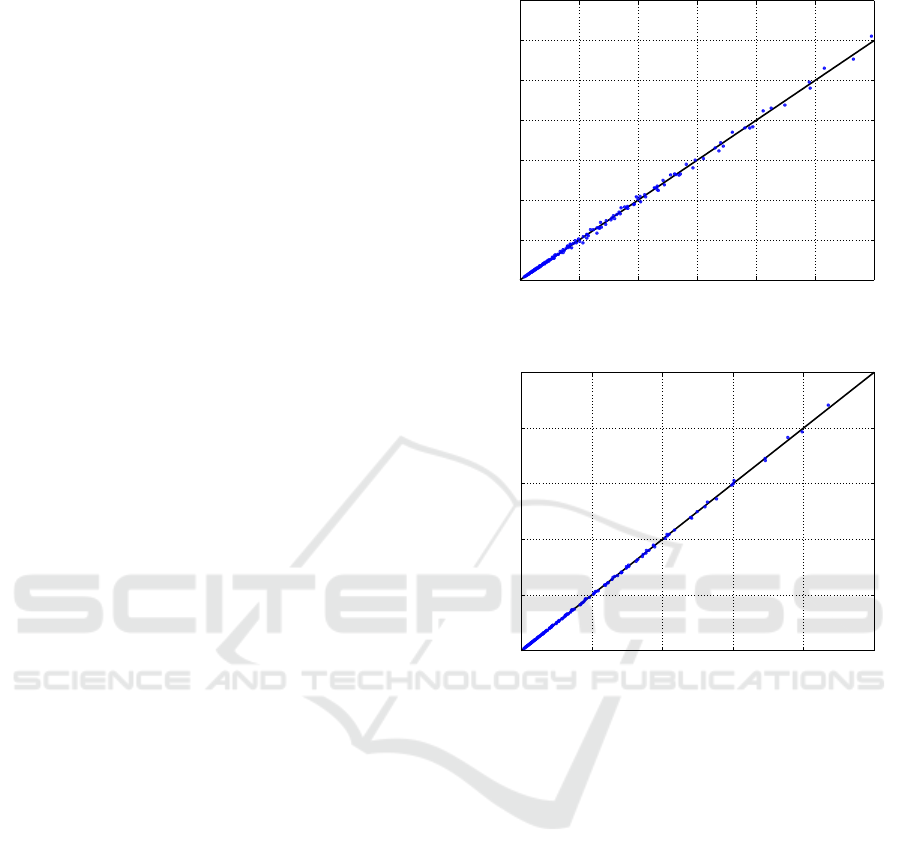
across the 160 data points, the MAPE settles at 2.94%
0
0
20
20
40
40
60
60
80
80
100
100
120
120
140
Predicted [s]
Actual [s]
AlexNet
Figure 1: AlexNet actual vs. predicted.
0
0
100
100
200
200
300
300
400
400
500
500
Predicted [s]
Actual [s]
GoogleNet
Figure 2: GoogLeNet actual vs. predicted.
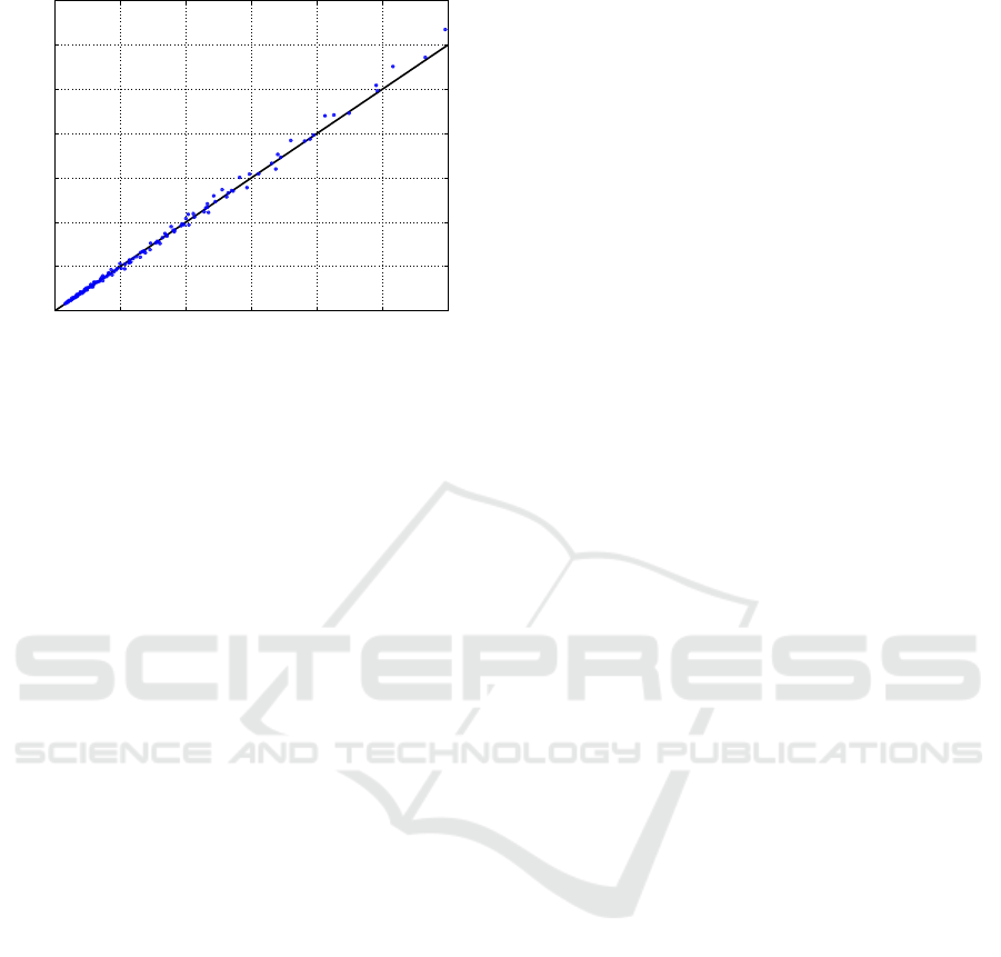
for AlexNet, 0.97% for GoogLeNet, and 1.53% for
VGG-16. Vice versa, the per layer models achieved
relative errors below 10% on average and were below
23% in the worst case. See (Gianniti et al., 2018) for
further details. Figures 1, 2 and 3 show the actual vs.
predicted plots for these three models. In line with
the accuracy suggested by the MAPEs, in all the three
plots the blue points lie very close to the black diago-
nal.
In order to assess the quality of execution time
prediction when extrapolating to higher parameter
ranges, for each CNN we split the dataset into train-
ing and test portions. Models were learned on the
subset devoted to the training phase, while the final
accuracy metric is the MAPE evaluated on the test set
by comparing overall real execution times with corre-
sponding predictions. By splitting the dataset we can
quantify the predictive capability on configurations
not available during the learning via linear regression,
particularly in terms of extrapolation towards larger
batch sizes and more overall iterations. This approach
to splitting data is motivated by the economic benefit
Performance Prediction of GPU-based Deep Learning Applications
283
Table 2: CNN Characteristics, Batch Size 1.
Network Layers Weights Activations Complexity
AlexNet 8 6.24E+7 1.41E+6 3.42E+9
GoogLeNet 22 1.34E+7 6.86E+6 4.84E+9
VGG-16 16 1.38E+8 1.52E+7 4.65E+10
Table 3: Operation Count and Layer Time Breakdown.
Network Category c
fw
l
[%] t
fw
l
[%] c
bw
l
[%] t
bw
l
[%]
AlexNet Conv/FC 99.51 83.11 99.66 80.29
AlexNet Norm 0.21 5.16 0.17 3.95
AlexNet Pool 0.10 5.36 0.05 10.94
AlexNet ReLU/Drop 0.19 6.37 0.12 4.82
GoogLeNet Conv/FC 98.33 69.80 98.94 67.67
GoogLeNet Norm 0.25 2.62 0.20 2.09
GoogLeNet Pool 0.82 16.35 0.46 22.18
GoogLeNet ReLU/Drop 0.60 11.23 0.40 8.07
VGG-16 Conv/FC 99.70 89.23 99.80 88.56
VGG-16 Pool 0.04 2.50 0.02 6.04
VGG-16 ReLU/Drop 0.26 8.27 0.17 5.40
0
0
500
500
1000
1000
1500
1500
2000
2000
2500
2500
Predicted [s]
Actual [s]
VGG-16
Figure 3: VGG-16 actual vs. predicted.
Table 4: End to End Model Validation, NVIDIA Tesla
P100-PCIe.
Network
˜
b ˜ı n
train
n
test
MAPE [%]
AlexNet 16 150 6 140 3.18
AlexNet 24 170 12 140 6.43
AlexNet 32 200 20 140 3.01
GoogLeNet 16 150 6 140 5.79
GoogLeNet 24 170 12 140 1.09
GoogLeNet 32 200 20 140 2.43
VGG-16 16 150 6 140 3.70
VGG-16 24 170 12 140 2.20
VGG-16 32 200 20 140 3.41
of running only a limited number of small scale exper-
iments, rather than spanning the whole domain where
parameters can attain values.
PSfrag replacements
Iterations
Batch size
Test
Train
Pred.
0
20
40
60
Execution time [s]
80
100
120
140
2000
2500
70
500
1000
1500
0
0
0
0
10
20
20
30
40
40
50
60
60
AlexNet — n
train
= 6
Figure 4: AlexNet end to end time, n
train
= 6.
Table 4 lists the results obtained with these exper-
iments. The split between training and test set was
performed by setting thresholds on the batch sizes and
numbers of iterations allowed in the former. Every
row corresponds to a model learned on the training
set {(b, i) ∈ B × I : b ≤
˜
b, i ≤ ˜ı}, whose sample size is
n
train
. For ease of comparison, we used as test set only
the subset of data points that do not appear in any of
the training sets, hence each CNN is associated with
a single test sample size n
test
. All the three CNNs
show good accuracy on the test set, with a worst case
MAPE of 6.43% even when rather small training sets
are used.
Figure 4 reports, as example, a plot depicting the
results obtained with the model learned for AlexNet
using the 6-element training set, which corresponds
to the first row in Table 4. Triangles represent the
CLOSER 2019 - 9th International Conference on Cloud Computing and Services Science
284
0
0
20
20
40
40
60
60
80
80
100
100
120
120
140
Predicted [s]
Actual [s]
AlexNet — n
train
= 6
Figure 5: AlexNet actual vs. predicted, test set, n
train
= 6.
data points in the training set, circles are real measure-
ments in the test set, while crosses are the predictions
given by the linear regression model. The predicted
execution times show a good accordance with the cor-
responding measurements, with a MAPE of 3.18% on
the test set. With this training set, the estimated coef-
ficients are in the order of magnitude of 10
−2
for
ˆ
β
i
and
ˆ
β
b
, while
ˆ
β
ib
is in the order of 10
−3
. As the batch
sizes b are typically between 10 and 100 and the num-
ber of iterations i are typically larger than 10000, the
dominant term will be i ·
ˆ
β
i
+ i · b ·
ˆ
β
ib
. This outcome
is quite intuitive, since, as discussed previously, the
product i · b quantifies the total number of images fed
into the CNN for processing: the amount of input data
has a major role in determining performance.
In order to provide further intuition on the accu-
racy of the proposed end to end modeling method,
Figure 5 shows the actual vs. predicted plot for test set
data points. The model is again learned for AlexNet
on the training set with n
train
= 6, thus the results
are consistent with Figure 4 and the first row of Ta-
ble 4. This figure allows for visually assessing predic-
tion accuracy, indeed all the blue dots gather closely
around the diagonal, plotted with a solid black line,
proving that prediction errors are small all across the
test set. The behavior in extrapolation remains quite
similar to what observed in Figure 1, where training
could exploit the full data set.
5 CONCLUSION
In this paper we discussed complementary modeling
approaches to predict the performance of DL tech-
niques based on CNNs. When the focus is on gen-
erality, the per layer models devised in our previous
work enable prediction with less than 10% on aver-
age and 23% worst case relative error even when ap-
plied to networks never seen during training, thanks to
their gray box approach. On top of their generaliza-
tion capability, these models also provide insights into
the performance characteristics of CNNs, which we
highlighted in the experimental section. Furthermore,
when users already settled on a specific network, it is
possible to achieve higher accuracy, with errors as low
as 2%, by switching to end to end models and trading
off generality for improved precision.
ACKNOWLEDGEMENTS
Eugenio Gianniti and Danilo Ardagna’s work has
been partially funded by the ATMOSPHERE project
under the European Horizon 2020 grant agree-
ment 777154.
REFERENCES
Baghsorkhi, S. S., Delahaye, M., Patel, S. J., Gropp, W. D.,
and Hwu, W.-m. W. (2010). An adaptive performance
modeling tool for GPU architectures. In PPoPP, vol-
ume 45, pages 105–114.
Bahdanau, D., Cho, K., and Bengio, Y. (2014). Neural ma-
chine translation by jointly learning to align and trans-
late. CoRR, abs/1409.0473.
Bahrampour, S., Ramakrishnan, N., Schott, L., and Shah,
M. (2015). Comparative study of Caffe, Neon,
Theano, and Torch for deep learning. CoRR,
abs/1511.06435.
Barnes, B. J., Reeves, J., Rountree, B., De Supinski,
B., Lowenthal, D. K., and Schulz, M. (2008). A
regression-based approach to scalability prediction. In
ICS, pages 368–377.
Bitirgen, R., Ipek, E., and Martinez, J. F. (2008). Coordi-
nated management of multiple interacting resources in
chip multiprocessors: A machine learning approach.
In MICRO.
Dao, T. T., Kim, J., Seo, S., Egger, B., and Lee, J.
(2015). A performance model for GPUs with caches.
26(7):1800–1813.
Gianniti, E., Zhang, L., and Ardagna, D. (2018). Perfor-
mance prediction of GPU-based deep learning appli-
cations. In SBAC-PAD.
Gupta, U., Babu, M., Ayoub, R., Kishinevsky, M., Paterna,
F., Gumussoy, S., and Ogras, U. Y. (2018). An on-
line learning methodology for performance modeling
of graphics processors.
Hadjis, S., Zhang, C., Mitliagkas, I., and Ré, C. (2016).
Omnivore: An optimizer for multi-device deep learn-
ing on CPUs and GPUs. CoRR, abs/1606.04487.
Hong, S. and Kim, H. (2009). An analytical model for a
GPU architecture with memory-level and thread-level
parallelism awareness. In ISCA, volume 37, pages
152–163.
Performance Prediction of GPU-based Deep Learning Applications
285

Jia, W., Shaw, K. A., and Martonosi, M. (2012). Stargazer:
Automated regression-based GPU design space explo-
ration. In ISPASS. IEEE.
Kerr, A., Diamos, G., and Yalamanchili, S. (2010). Model-
ing GPU-CPU workloads and systems. In GPGPU-3.
ACM.
Krizhevsky, A., Sutskever, I., and Hinton, G. E. (2012). Im-
ageNet classification with deep convolutional neural
networks. In NIPS.
Lin, M., Chen, Q., and Yan, S. (2013). Network in network.
CoRR, abs/1312.4400.
Liu, W., Muller-Wittig, W., and Schmidt, B. (2007). Perfor-
mance predictions for general-purpose computation
on GPUs. In ICPP. IEEE.
Lu, Z., Rallapalli, S., Chan, K., and La Porta, T. (2017).
Modeling the resource requirements of convolutional
neural networks on mobile devices. In MM. ACM.
Luk, C.-K., Hong, S., and Kim, H. (2009). Qilin: Ex-
ploiting parallelism on heterogeneous multiprocessors
with adaptive mapping. In MICRO. ACM.
Madougou, S., Varbanescu, A., de Laat, C., and van Nieuw-
poort, R. (2016). The landscape of GPGPU perfor-
mance modeling tools. J. Parallel Computing, 56:18–
33.
Sainath, T. N., Kingsbury, B., Saon, G., Soltau, H., Mo-
hamed, A., Dahl, G. E., and Ramabhadran, B. (2015).
Deep convolutional neural networks for large-scale
speech tasks. Neural Networks, 64.
Simonyan, K. and Zisserman, A. (2015). Very deep convo-
lutional networks for large-scale image recognition. In
ICLR.
Song, S., Su, C., Rountree, B., and Cameron, K. W.
(2013). A simplified and accurate model of power-
performance efficiency on emergent GPU architec-
tures. In IPDPS. IEEE.
Srivastava, N., Hinton, G. E., Krizhevsky, A., Sutskever, I.,
and Salakhutdinov, R. (2014). Dropout: A simple way
to prevent neural networks from overfitting. JMLR,
15.
Szegedy, C., Liu, W., Jia, Y., Sermanet, P., Reed, S.,
Anguelov, D., Erhan, D., Vanhoucke, V., and Rabi-
novich, A. (2015). Going deeper with convolutions.
In CVPR. IEEE.
Venkataraman, S., Yang, Z., Franklin, M. J., Recht, B., and
Stoica, I. (2016). Ernest: Efficient performance pre-
diction for large-scale advanced analytics. In NSDI.
Vincent, P., Larochelle, H., Lajoie, I., Bengio, Y., and Man-
zagol, P. (2010). Stacked denoising autoencoders:
Learning useful representations in a deep network
with a local denoising criterion. JMLR, 11.
Wang, Y., Zhang, L., Ren, Y., and Zhang, W. (2017). Nexus:
Bringing efficient and scalable training to deep learn-
ing frameworks. In MASCOTS.
Zhang, Y. and Owens, J. D. (2011). A quantitative per-
formance analysis model for GPU architectures. In
HPCA. IEEE.
CLOSER 2019 - 9th International Conference on Cloud Computing and Services Science
286
