Minimization of Attack Risk with Bayesian Detection Criteria
Vaughn H. Standley, Frank G. Nuño and Jacob W. Sharpe
College of Information and Cyberspace, National Defense University, 300 5th Ave., Washington D.C., U.S.A.
{vaughn.standley.civ, frank.g.nuno.mil, jacob.w.sharpe.civ}@ndu.edu
Keywords: Complex Systems, Bayesian Minimization, Deterrence, Likelihood Ratio, Power-law, Log-normal,
Log-gamma.
Abstract: Strategic deterrence operates in and on a vast interstate network of rational actors seeking to minimize risk.
Risk can be minimized by employing a likelihood ratio test (LRT) derived from Bayes’ Theorem. The LRT
is comprised of prior, detection, and false-alarm probabilities. The power-law, known for its applicability to
complex systems, has been used to model the distribution of combat fatalities. However, it cannot be used as
a Bayesian prior for war when its area is unbounded. Analytics applied to Correlates of War data reveals that
combat fatalities follow a log-gamma or log-normal probability distribution depending on a state’s escalation
strategy. Results are used to show that nuclear war level fatalities pose increasing risk despite decreasing
probability, that LRT-based decisions can minimize attack risk if an upper limit of impending fatalities is
indicated by the detection system and commensurate with nominal false-alarm maximum, and that only
successful defensive strategies are stable.
1 INTRODUCTION
Reflecting on how much the world and warfare have
changed, famed political scientist Sir Lawrence
Freedman observed that “there is no longer a
dominant model for future war, but instead a blurred
concept and a range of speculative possibilities”
(Freedman, 2017). Strategists and politicians have
proven unimpressive in predicting the circumstances
and outcomes of wars, and the international arena has
only become more complex. With the aim of
maintaining peace, scholars and practitioners will
over time narrow the possibilities and bring the
concept of war into focus. Meanwhile, some truths
will remain invariant. Among them, nations make
decisions based on likelihoods derived from past
experiences, not on mere reasoned possibilities. And
despite the differences between, say, the Russo-
Japanese War and a future nuclear war, they will be
inextricably linked by at least one quantitative
measure: combat fatalities.
War is by no means a solely rational endeavour.
Nevertheless, when faced with the prospect of
expending resources and lives, possibly risking its
very existence, nation states will attempt to weigh the
consequences of action and inaction in order to
minimize risk. Given the uncertainties described by
Freedman, the immense potential death toll of nuclear
war, and human propensity for error under duress,
understanding risk when considering evidence that an
attack is imminent or underway is essential to sustain
the two “grounds for making peace: the first is the
improbability of victory; the second is its
unacceptable cost” (von Clausewitz, 1976)
The power-law of statistics, known for its
applicability to complex systems (Sornette, 2007),
has been used since the 1950s to study violent conflict
(Richardson, 1960). A phenomenon may be
probabilistically distributed according to the power-
law if the logarithm of the exceedance probability
plotted against the logarithm of severity s
appears as a straight line with a negative slope –q.
Intuitively this means that the probability of
exponentially increasing consequences is decreasing
exponentially. However, researchers consistently
report that the power-law’s exponential parameter q
for the severity of war measured in deaths is less than
one, indicating that the exceedance probability
decreases slower than the increase in number of
deaths. Given that risk is probability multiplied by
consequences, this means that the risk of war forever
increases for increasing fatalities. It is a condition that
makes the power-law invalid as a probability
distribution because the area under the
curve is unbounded and the mean is divergent.
Military deterrence is a function of rational actors
seeking to minimize military risk within a vast and

adversarial international system. These actors can
minimize risk by applying a likelihood ratio test
(LRT), derived from a dichotomous form of Bayes’
Theorem, to a series of hypothesis tests weighing the
risk of action versus inaction. Before applying an
LRT, however, there must be a probability on which
to base the test. For war, the power-law cannot be
used given that 1. The aim of this research is to
identify a valid probability for the severity of war that
could be used in a Bayesian-derived LRT, and then
draw conclusions advancing the field of strategic
deterrence, with particular focus on detection and
false-alarm probabilities in the context of attack
warning.
2 RISK-INFORMED DECISIONS
Risk-informed decision-making requires the ability to
prioritize decisions according to their quantitative
risks. The field of probabilistic risk assessment has
over the years led to a standard definition of risk,
which is the expected cost of an event equal to the
sum of the products of the consequences multiplied
by their probabilities (Advisory Committee on
Reactor Safeguards, 2000). The simplest risk-
informed decision involves dichotomous outcomes,
where the risk of two mutually exclusive choices are
weighed against each other and the lower risk of the
two is selected (i.e. dichotomous hypothesis testing).
Decisions about dichotomous events “” and “
̅
”
can be made by comparing risks
and
̅
̅
̅
, respectively, where
is the cost of
not countering and
̅
is the cost of countering
̅
.
In this analysis, negative risks (i.e. profit, gain, etc.)
are not considered. We call these “prior risks”
because they rely on the prior probability . And
as there are only two choices,
̅
1.
Event could be nearly anything. In this paper it
represents an “attack” and
̅
represents “no attack”.
One chooses to believe an attack is the outcome if
̅
, also written as follows:
̅
̅
(1)
This formulation indicates when it is favourable to
attack without detection or intelligence. Health
insurers, for example, set premiums based solely on
prior probability when they are not allowed to
consider an individual’s specific pre-existing
conditions that is normally detected by a test (Sox et
al., 2013). Given the multitude of detection
capabilities fielded by most states today, use of
equation (1) in isolation is not realistic. However, the
computation of these risks represents a necessary step
leading to decisions that take into account detection
systems. The next step in this progression leads to Eq.
(2), which is a dichotomous form of Bayes’ theorem
that includes the probability of detection | and
the probability of false-alarm |
̅
:
|
̅
|
|
|
̅
̅
(2)
The left-hand side of Eq. (2) is the ratio of the
posteriors. Given datum , attack is more likely than
not if the right-hand side of Eq. (2) is greater than one.
Notwithstanding the costs, |/|
̅
must be
greater than
̅
/ and also greater than one.
Costs are factored in by replacing the prior
probabilities with the prior risks as in Eq. (3), leading
to a likelihood ratio test (LRT):
|
|
̅
̅
(3)
We call the left-hand side of Eq. (3) the likelihood
ratio, L, and the right-hand side the critical likelihood
ratio, L*. Risk is minimized when the decision is
made in accordance with the LRT. Specifically, if the
LRT is true, then L is greater than L*, and one takes
action based on the belief that an attack is real.
Otherwise, no action is taken. Equations (1) and (3)
are thus our models for rational behaviour, with and
without detection, respectively.
3 DATA ANALYTICS
Risks in equations (1) and (3) will be per year per
target state or alliance as derived from the Correlates
of War (COW) Project historic war datasets (Sarkees,
2010). For illustrative purposes, North Atlantic
Treaty Organization (NATO) states are arbitrarily
chosen to be the collective target of attack.
3.1 Dataset Typology
The COW Project has published a traditional and
expanded typology of war. We use the latter. COW’s
Inter-State classification of wars is based upon the
status of territorial entities, focusing on those that are
classified as members of the state system. This dataset
encompassing wars that took place between or among
recognized states where there are at least 1,000
fatalities. COW’s Extra-State classification of wars
involves imperial and colonial wars. The Intra-State
classification of wars encompasses different kinds of
wars that take place predominantly within the
recognized territory of a state. The last category, Non-
State wars, involve non-state territory or across state
borders. COW war data exists as rows of named wars
that include start and end dates, combat deaths,
outcome, and little else. A state’s population during a
war, for example, is in a different dataset. We analyse
only the data available in the COW war datasets.
The focus of this study is strategic war, which
requires a level of resources achievable only by states.
Therefore, only inter- and/or intra-state war data seem
applicable, so the other datasets are not used. From
1816-2007 there are 91 and 199 Inter- and Intra-State
wars, respectively.
3.2 Temporal Prior Probability
The short treatment of temporal probability that
follows is simplistic. We use it, nevertheless, because
of its illustrative value and because it quickly
becomes apparent that the severity of war is much
more important to arriving at risk-informed decisions
than is temporal probability.
For the prior probability of attack, , we begin
by using the temporal statistics of the COW Inter-
State war dataset. The time between wars is
exponentially distributed where there is on average
about one interstate war every two years, yielding an
exponential distribution parameter 0.5/.
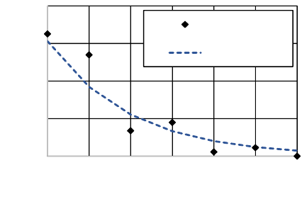
The exponential distribution is fit to the data in Figure
1. The fit has an r
2
value equal to 0.93, indicating a
good fit. Equivalently, the probability of there being
one or more wars per year follows the Poisson
distribution with the same parameter. Thus, in any
given year there is a 31% chance that one war will
occur somewhere in the world.
Figure 1: Exponential distribution fit (=0.51 wars/yr) to
COW Inter-State war data where fit goodness r
2
=0.93.
About 62% of the states are defensive in the wars
(see Table 1). And, because 46% of the wars
comprising this data involved countries that are today
part of NATO, there is approximately a 0.31
0.62 0.46 0.088 probability each year that
NATO will be attacked once. The average deaths and
number of states participating in wars has remained
nearly constant in the last 200 years. Thus, additional
temporal changes across datasets do not warrant
further consideration.
3.3 Severity Probability
The severity of war is needed to estimate
, which is
necessary to compute the risks in equations (1) and
(3). Previous research suggests that severity is
probabilistic, in which case
is equal to severity s
times the probability that a war of severity S is equal
to s, conditional on if an attack has occurred. This
is written as |. Severity has also been
modelled as s multiplied by the exceedance
probability, which we write here as |.
3.3.1 Power-law
Lewis Fry Richardson was the first to plot the
logarithm of the frequency of deaths in violent
conflict against the logarithm of their severity,
revealing a straight line with a negative slope,
suggesting the applicability of power-law statistics
(Richardson, 1960). Exceedance probabilities are
obtained simply by dividing the frequencies by the
total number of conflicts. Cederman affirmed
Richardson’s work using COW data and reports a
slope of negative 0.41 (Cederman, 2003). However,
Cederman’s log-log plot displays a slight curvature in
the vicinity of 1,000 and 10,000 deaths. This
curvature may indicate that the power-law is not the
best distribution to be applied, that there is
insufficient data, that the wrong kind of data has been
used, or that a combination of these errors applies.
Pursuing a hunch that more data is needed to
obtain a valid power-law result, we combined the
COW Inter-State and Intra-State datasets, obtaining
in this case a value of q=0.70 with an r
2
of 0.99. This
result is shown as the dashed orange line in Figure 2.
The red-dashed line is for q=1, indicating the smallest
valid q value. Above this line, the power-law is
invalid as a probability distribution. Consistently,
researchers report values that are less than one, ours
included. Having proved the hunch incorrect, we
sought to apply another probability distribution.
3.3.2 Log-normal Distribution
The curvature seen in the power-law fits suggest that
the log-normal distribution might be better suited to
model the data (Benguigui and Marinov, 2015).
0
0.1
0.2
0.3
0.4
1234567
P(T=t)
YearsBetweenConsecutiveWars
COWData
Exp.Dist.Fit
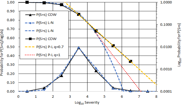
However, because the COW Inter-State data only
includes wars having a minimum of 1000 deaths, it is
also necessary to combine Inter- and Intra-State
dataset, thus providing statistics below this minimum.
A log-normal (
= 3.6,
= 0.81) density function
is seen to closely follow the data. This is
indicated by the blue-dashed, bell-shaped curve in
Figure 2. COW data is indicated by the black line with
black triangles. The r
2
obtained by comparing these
two curves is 0.99, indicating an excellent fit.
To highlight the small differences in cases of wars
exceeding one million deaths, an expected result in
any nuclear conflict, exceedance probability curves,
P(S > s), are included. In Figure 2 the log-normal
exceedance probability is the blue-dashed curve
above the probability density functions following the
logarithmic scale on the right side of the graph. COW
data is indicated by a black curve with black squares.
The log-normal fit fails to match the COW data for
high death totals. This result is in contrast to the
extremely good fit provided by the power-law.
Despite the overall excellent fit of the log-normal,
we are motivated to seek an alternative method that
better fits the high severity data. The excellent fit to
this data by power-law, even in the case of combining
the Inter- and Intra-State datasets, indicates that there
is an underlying phenomena favouring higher
severity. The log-normal distribution is a symmetric
distribution that does not favour upper statistics. Use
of the log-gamma distribution, however, may solve
this problem as it is an asymmetric distribution that
favours the higher range (Halliwell, 2018).
3.3.3 The Effect of Alliances
Combining Inter- and Intra-State datasets creates a
dataset with deaths below 1000, enabling log-normal
fit with a high r
2
value, but it fails to enable a fit the
high-magnitude war data points. Mixing these data
sets may add error to the analysis.
Figure 3 is a plot of the base-10 logarithm of
deaths versus the number of allies in the named
interstate wars. It appears that part of the interstate
war data correlates with the number of alliances.
However, all of the data cannot be satisfactorily fit
using a single exponential line. The best fit to all of
the data is poor (r
2
=0.1943). The best fit to the wars
involving five or less participants, the blue dots, is
extremely poor (r
2
=0.0552). The best fit to wars
having greater than five participants, marked with red
dots, begins to show some correlation (r
2
=0.5672). A
partial correlation can only adversely affect the
statistics and obfuscate a more applicable probability
distribution. Therefore, we ungroup the Inter-State
dataset so that deaths are not the total of named wars
for all allies. Ungrouping also creates a larger dataset
that includes deaths below 1,000. The number of wars
also increases from 91 to 319 and more than half of
the wars have less than 10,000 fatalities.
Removing the named-war grouping helps with
data analysis, but its potential significance is also
worth discussing. Jackson and Nei reported that there
were ten times fewer wars between 1950 and 2000 as
a result of political, military, and economic alliances
(Jackson and Nei, 2015). In other words, peace and
war are at least partly the result of a network
phenomenon.
Figure 2: Power-law (P-L) and log-normal (L-N) fit to COW Inter- and Intra-State war datasets.
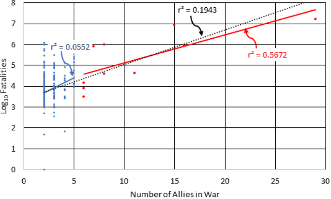
Figure 3: Inter- and Intra-State COW dataset deaths versus the number of states indicate an inconsistent effect caused by
alliances, where r
2
for 2 to 5 state wars is very weak (0.055, blue dots and blue line), moderately good for 6 – 29 states (0.57,
red dots and red line), and weak for the combined data (0.19, black dashed line).
In the instant case, however, removing the effect of
alliances helps better understand the state
individually as a rational actor.
3.3.4 Log-gamma Distribution
As with the log-normal, the log-gamma is a
distribution of the log of datum. Probability density
functions derived from both COW data and a log-
gamma distribution (
= 9.0,
= 0.39) are indicated
in Figure 4. The fatalities used to derive the curves
are from individual rows in the Intra-State dataset, not
the sum of fatalities for respective named wars
involving multiple states. The r
2
of the log-gamma fit
compared to the COW data is 0.99, indicating an
excellent fit. Equally important, the log-gamma fit
holds for s > 10
6
. This is indicated by the exceedance
probability curve that follows the logarithmic scale on
the right-side of Figure 4. A side effect of de-
grouping named wars is that the maximum number of
deaths experienced for a given war does not exceed
10
7
. Furthermore, because the P(S>s) curve follows
the complement of the integral of P(S=s), there is no
data points for P(S>10
7
). To check the fit for these
high values, we compare the average slope of the
power-law and log-gamma curves between P(S>10
4
)
and P(S>10
8
). We find them in good agreement (0.62
versus 0.55). Thus, the log-gamma distribution fits
the entire range of severity covered by the COW data
when the wars are analysed only by nation state. The
slope of the log-gamma increases in negativity,
however, so that the distribution is valid for higher
death values. Specifically, the slope of the P(S>s)
curve between 10
8
and 10
9
is log1.110
9.510
3.0. As this slope is less than
negative one and decreasing, the fit is valid.
4 RISK MINIMIZATION
Keeping peace requires that states not take undue
action while avoiding inaction that might invite
attack. This delicate balance can be optimized by
minimizing expected combat deaths, taking into
account attack detection and false-alarm
probabilities, which we can now do using prior
probabilities that span both conventional and nuclear
levels of fatalities. Exactly how and why becomes
clearer in the presence of a game-theoretic model of
war, which we provide first and then incorporate into
a likelihood-ratio analysis. It is then reasonable and
practical to assume that the probability of detection is
exactly one. Most detection systems provide nearly
this level of performance and the assumption leads to
a single risk of inaction with and without detection,
which makes more tractable an analysis of the impact
of false-alarm probability on attack decisions.
4.1 Game-theoretic Analysis
Figure 5 shows the win-loss distribution of deaths for
attackers and defenders from the un-grouped Inter-
State dataset based on COW’s assessment of what
constitutes “win” and “lose”.
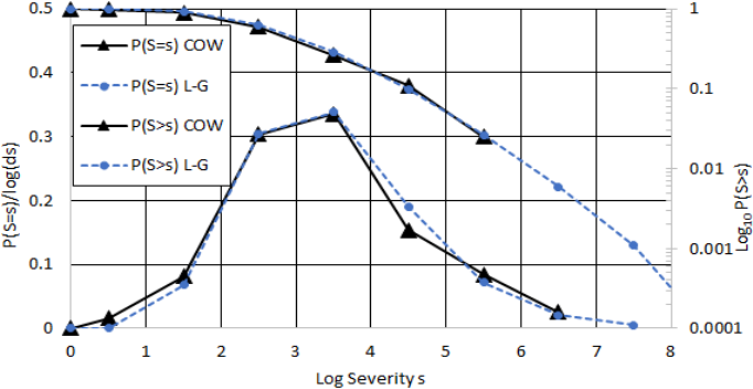
Figure 4: COW Inter-State war and log-gamma (L-G) probability density curves, P(S=s), and exceedance probability curves,
P(S>s), where density curves track the left-side scale and the exceedance curves track the right-side scale.
Key information from this graph is summarized in
Table 1. The “Other” category in Table 1 includes
ties, transformations, and stalemates. The percentages
are the number of wars in the category divided by the
total number of wars, where the total for the six
categories is 100%.
Table 2 reconciles the “max deaths” information
in Table 1 with game-theoretic strategies. Given that
an attack has already occurred, we hypothesize that
attackers and defenders have two available strategies:
“escalate” and “deescalate.” Both take into account
the strength of a state’s motives and resources. Thus,
use of the deescalate strategy may be the result of
previous escalation having depleted the state’s
national will and resources. The maximum deaths
experienced by a state is chosen to be the limit of
losses a state would accept in a war for the particular
strategy. For example, given that 7.5M is the
maximum loss a state (U.S.S.R. in WWII) has
endured by way of defensive escalation, this is taken
to be the maximum loss for the strategy. Conversely,
3.5M is the maximum loss of an attacker (Germany
in WWII) endured via offensive escalation.
Maximum losses for other strategies are similarly
derived.
The game-theoretic model of Table 2 leads to two
Nash Equilibrium points (Nash, 1950), one at
escalate-deescalate, the other at deescalate-escalate.
These equilibrium points are consistent with the fact
that wars, once started, normally escalate and result
in high losses no matter if the attacker or defender is
the winner. The escalate-escalate cell is not an
equilibrium point because mutual escalation leads to
losses that are greater than losses in adjacent cells.
Eventually, conflicts move to escalate-deescalate or
deescalate-escalate where a winner and loser
eventually emerge. The deescalate-deescalate cell is
normally unstable, which is why only 18% of the
wars end in this state.
The strategies in Table 2 are also consistent with
the distributions of war severity. Escalation or
deescalation is a multiplicative increase or decrease
in the expense of human resources. Where
is a
random variable representing the fractional increase
or decrease of combatants during each escalation or
deescalation, severity is random variable equal to the
products of these changes,
~
…
,
resulting in the applicability of a logarithmic
distribution. In other words, leaders escalate or
deescalate based on the quantity of deaths already
incurred. Relative increases or decreases follow a
logarithmically distributed process (Ott, 1990).
Noting that gamma and Poisson distributions are
conjugates, what is more challenging to understand is
why three of the win-lose distributions in Figure 5
appear to be log-gamma distributions (~L-G), but
only the defend-win curve appears to follow a log-
normal distribution (~L-N). The defend-win category
is comprised of far greater losses than any other
category (i.e. 17M versus 6.4M for defend-lose, 5.4M
for attack-lose, and 0.8M for attack-win).
Symmetry of the defend-win distribution may
indicate that there are underlying random variables
that are not strictly positive numbers as are fatalities.
Economy and infrastructure are examples of variables
that could also be negative and whose effect might be
in play. More likely, a defender who is escalating in
response to an attacker who is escalating increasingly
relies on the benefits of alliances as discussed in
section 3.3.3. Indeed, most of the fatalities associated
with the log-normal defend-win curve are from the
many allied countries in WWII.
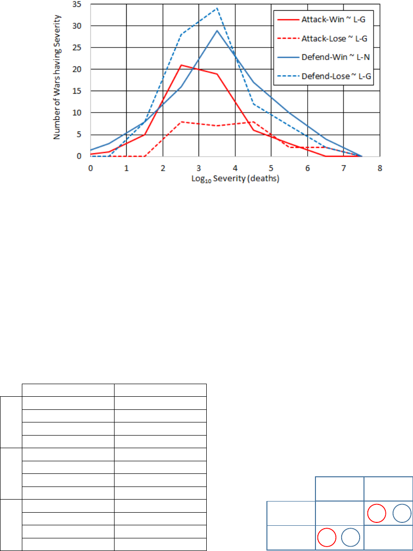
Figure 5: Attack-defend-win-lose distributions for wars as a function of the log of severity.
4.2 Minimization without Detection
Table 3 reports the annual risk of inaction for NATO
based on probabilities in Table 1 and Figure 5. Risk
is the severity probability in the row times the
midpoint of the range of deaths. The result is then
multiplied by 0.088, as estimated in section 3.2, to
calculate the risk per year for NATO. Numbers are
rounded to two significant figures. Two sets of
probabilities and two sets of risks are provided, one
from the COW data and the other based on the
defend-lose log-gamma fit.
Table 1: Attack-Defend-Win-Lose statistics, based on
COW definitions, and parametric fits to the data.
Attack(38%) Defend(62%)
Win(44%)
17% 27%
0.25Mmaxdeaths 7.5Mmaxdeaths
L-G(10,0.32)r
2
=0.99 L-N(3.5,1.2)r
2
=0.95
=2.9,=0.99 =3.5,=1.2
Lose(38%)
9% 29%
3.5Mmaxdeaths 1.8Mmaxdeaths
L-G(8.0,0.48)r
2
=0.88 L-G(11,0.31)r
2
=0.97
=3.9,=1.1 =3.4,=1.0
Other(18%)
12% 6%
0.50Mmaxdeaths 0.75Mmaxdeaths
L-G(17,0.20)r
2
=0.84 L-G(12,0.24)r
2
=0.96
=2.8,=1.3 =3,=1.0
The rightmost columns are the “expected risk of
inaction” because they are the average number of
deaths that will result from war each year if nothing
is done. Given the exponential scale, the data and
model agree reasonably well until the data ends.
Although we don’t distinguish between deaths from
conventional or nuclear weapons, the number of
deaths resulting from nuclear weapons used in WWII
suggest that 100K or more deaths are nuclear-war-
level. What one can conclude from this table, then, is
that the risk of war increases for increasing ranges of
fatalities, making nuclear war the highest risk despite
decreasing in probability. This is true whether from
surprise attack or a slow build-up.
In the absence of a detection capability, risk-
informed decision can be made based only on the
prior probabilities in Table 3. A state may consider
attacking its foe to pre-empt an attack that it thinks is
probable. The predilection to attack, or the likelihood
of being attacked, would depend on the risk of action
weighed against inaction. Normally there will be
many scenarios for action, and each must be weighed
against inaction.
Table 2: Game model based on maximum win-loss deaths
(millions) with Nash Equilibria indicated (circled).
Pre-emptively attacking may reduce the number
of fatalities through destroying part of the enemy’s
attack capabilities. A rational NATO alliance would
do so only if the risk of action is less than the corres-
3.5,7.5
0.25,1.8
1.8,0.25 0.5,0.75
Escalate
Deescalate
Deescalate
Escalate
Defender
Attacker

Table 3: Annual risk of attack on NATO countries in expected deaths.
Severity
s
n
SeverityRange
s
n‐1
<Deads
n
Δs
=s
n
–s
n‐1
ProbabilityforSeverityRange ExpectedAnnualRiskofInaction
COWDefend‐Lose L‐GDefend‐lose BasedonData BasedonModel
10 1<Dead10 9 0.00 0.000016 0 0
100 10<Dead100 90 0.088 0.041 1 0
1K 100<Dead1K 900 0.31 0.30 24 23
10K 1K<Dead10K 9K 0.37 0.38 300 300
100K 10K<Dead100K 90K 0.13 0.20 1000 1,600
1M 100K<Dead1M 900K 0.077 0.066 6,100 5,300
10M 1M<Dead10M 9M 0.022 0.016 17,000 12,000
100M 10M<Dead100M 90M NoData 0.0029 NoData 23,000
1B 100M<Dead1B 900M NoData 0.00044 NoData 35,000
ponding row in Table 3. In the case of the row
designated “1M<Dead10M”, for example, the risk
of the pre-emptive attack would need to be less than
17K, based on data (12K modelled). Solving Eq. (1),
the maximum consequences of incorrect action is
̅
17,000 1 0.088/0.088 180,000. In
other words, if NATO were confident that no more
than 180K dead would result in a pre-emptive attack,
then the attack in this case is rational from a strictly a
fatalities perspective. Again, this scenario is
appropriate only if the alliance expects an attack.
4.3 Minimization with Detection
A pre-emptive strike based solely on prior probability
of combat deaths is not realistic given the many
detection systems fielded. However, computing the
risk of action and inaction per Eq. (1) is useful
because these quantities are needed in the right-hand
side of Eq. (3). Equation (4) below specifies the right-
hand side of Eq. (3), the Bayesian detection criteria,
using details from Table 1 (i.e. L-G, 11 and
0.31) where the consequence of action
̅
is the only
unknown quantity. Modelled severity, rather than
data, is used to enable a study of extreme conflict that
might cause between 10M and 1B fatalities:
∗
̅
1 0.088
∆ L-G
log
s
; 11,0.31
0.088
(4)
∗
from Eq. (4) can be used in Eq. (3) to study
possible decisions involving alert bomber forces, for
example, that can be launched on warning of attack
and recalled if there is a false-alarm. Alert forces must
be supported by a continuously functioning attack
detection system that is survivable through all
foreseeable conflicts. If NATO policy is to launch its
bombers upon warning of inbound ballistic missiles,
similar to U.S. policy (U.S. Dept. of Defense, 2018),
there are at least two possible outcomes with risks that
are defined in terms of detection and false-alarm: the
system fails to detect an actual attack, no action is
taken, resulting in the loss of the alert force and
fatalities proportional to the number of missiles; or
the system reports a false-alarm, prompting the
launch of the alert forces, causing the enemy to make
its own launch-on-warning decision. These two
outcomes are considered in turn using Eq. (4).
Being a number close to, but necessarily less than
one, the detection probability proportionally reduces
the threat that the NATO alert forces pose to an
enemy. This proportionally increases the threat of
attack by an opponent who has intelligence about the
detection probability or is capable of reducing it
through cyber- or information-operations. However,
because detection probabilities approach one and
false-alarm probabilities are normally much less than
one, the ratio of detection over false-alarm
probabilities is numerically dominated by the false-
alarm value. For this reason, it is correct and practical
to assign the probability of detection a perfect value
of one and assume that only the false-alarm
probability changes the likelihood ratio .
Table 4 reports
∗
as a function of
and
̅
.
NATO should launch its bombers if the likelihood
ratio of its detection system is greater than the
corresponding
∗
. However,
∗
cannot be less than
one or arbitrarily high. An value less than one
violates the basis on which Eq. (3) was derived. An
arbitrarily high implies a false-alarm probability
that is unachievably low. For example, a difficult-to-
achieve 0.001 false-alarm probability for Synthetic
Aperture Radar (Li, 1994) yields 1/
0.001 3. In Table 4, this and similar values are
coloured yellow indicating that it may be
unachievably low. Red cells indicate invalid or values
that are too low. Green cells indicate nominal values.
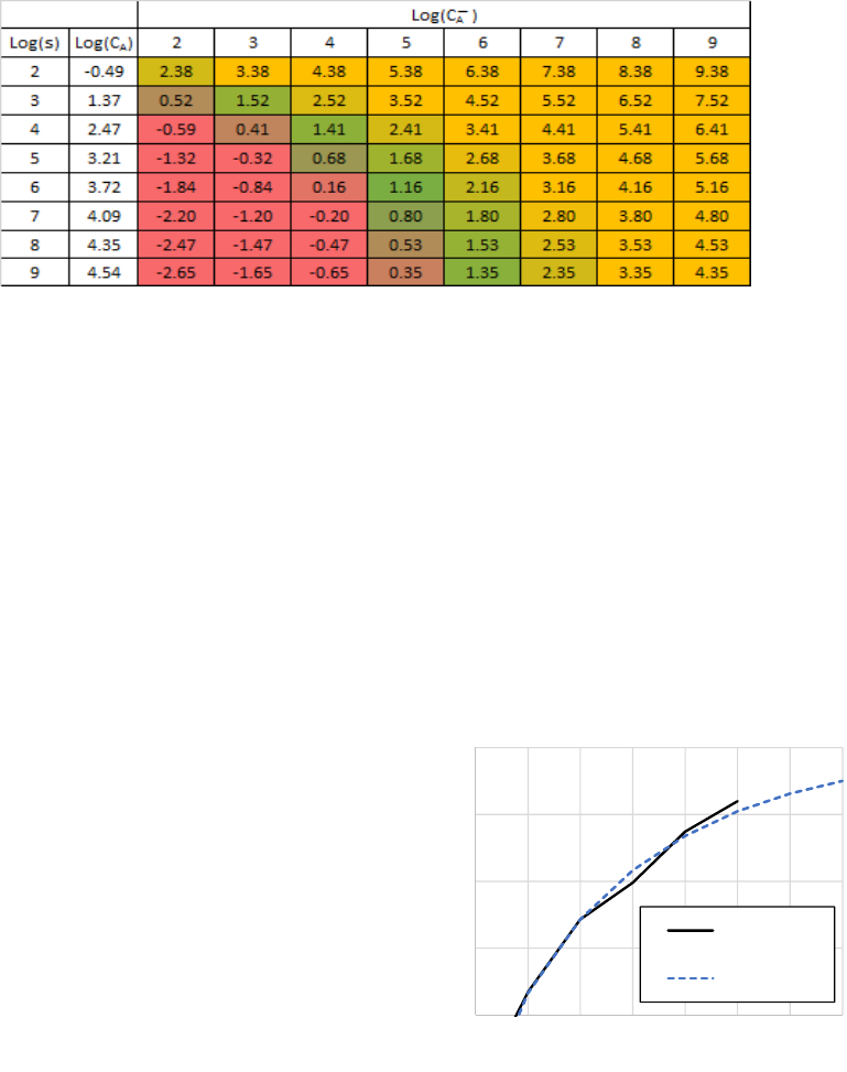
Table 4:
∗
as a function of
and
̅
, where red cells are invalid or too low, green contain normal and
useful values, and yellow indicates that the required false-alarm probabilities may be unrealistic.
The consequences of acting on a false-alarm are
potentially far more serious than the consequences of
inaction. For example, a technical glitch could result
in a full-scale nuclear war. Thus, deterrence is as
much about detection and false-alarm as it is about
the quantity and destructiveness of weapons.
Consider again the last row in Table 3 for which there
is COW data, marked “1M < Dead 10 M”, where
the data indicates a severity probability of 0.022 and
an annual risk to NATO countries equal to 17K
deaths. For this case, it would be rational for NATO
to take an action intended to negate war only if that
action resulted in annual risk less than 17K. One
example of such an action is to put strategic bombers
on alert so they can be launched before being
destroyed in a surprise attack. While this action may
have economic impact, it risks few NATO combatant
lives directly. So long as this action increases the
riskto the enemy for attacking, the enemy cannot
rationally choose to attack because the risk table
applies equally to them. Thus, the U.S.
Administration’s recent decision to put bombers back
on alert makes sense provided that the enemy is
confident their attack would be detected and that the
bombers could put at risk more of the enemy’s lives
than would be saved in a pre-emptive attack.
In all cases, robust and hardened detection and
alerting systems are paramount. These systems
require hardware, software, and human operators that
don’t automatically reject the possibility of a surprise
attack. Deterrence is also improved if detection
information is shared with the enemy because it helps
ensure they too will react correctly to alarms. If the
log-gamma model results are to be believed, even for
a just a few rows past the data, then the risk continues
to increase and the maximum false-alarm probability
rapidly decreases to unachievably small values. This
trend, partially seen in Figure 6, eventually reverses,
but well past the end of the table where human
population is exceeded. This result holds despite all
of the modelled uncertainties and is true even though
we have replaced the power-law with a distribution
that is probabilistically valid. The high risk behaviour
of war remains and it leads to the following
observation. A sufficiently low false-alarm
probability to justify a launch-on-warning decision is
not achievable if that decision results in an arbitrary
scale of retaliation. However, the same is not true if
the scale of the attack is known. For example, if
satellites are able to confirm that only ten missiles are
inbound and each can kill at most 1M, then the row
“1M < Dead 10M” applies and launch-on-attack is
rational for log-likelihood ratios equal to and greater
than 0.80. Referring to Table 4, these are cells in the
4.09 row, to the right of the
̅
4 column.
Figure 6: Log of attack risk vs. log deaths.
One can now make sense of power-law results by
computing pseudo q-values based on the log of the
slope of the upper end of exceedance probabilities for
the log-normal and log-gamma fits. The only strategy
with a pseudo q-value greater than one corresponds to
the log-normally distributed defend-win case. See
1
2
3
4
5
23456789
LogRisk
LogDeaths
COW
Log‐Gamma
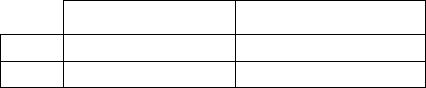
Table 5 below. Thus, for high-magnitude war only
defensive strategies generate bounded results.
Table 5: Pseudo q-values for log-gamma and log-normal
exceedance probabilities based on indicated COW deaths.
Attacker(s) Defender(s)
Win q=0.83,0.8Mtotal q=1.2,17Mtotal
Lose q=0.5,5.4Mtotal q=0.78,6.Mtotal
5 CONCLUSION
Risk of military attack, in terms of combat fatalities,
can be minimized using a Bayesian detection criteria
based on prior probability distributions derived from
COW Inter-State war data. Use of the power-law in
this context is invalid and should be abandoned. A
game-theoretic model with two Nash Equilibrium
points help explain why combatant fatalities follow a
log-gamma or log-normal probability distribution
depending on if a state is offensive or defensive. De-
correlating combat fatalities from alliance effects
exposes the log-gamma structure of the defend-lose
case and enables a calculation of attack risk per year
for ranges of deaths in powers of ten. Further, the data
indicate that war occurs with predictable temporal
frequency where the likelihood of one or more wars
in a year follows the Poisson distribution. After being
initiated, a war escalates or deescalates proportional
to the combat losses already incurred. The data also
shows that the risk of nuclear war level fatalities
increases despite decreasing in probability. Taking
into account detection and false-alarm probabilities,
an LRT advises that it is rational to escalate only
when the consequence of inaction and action are
about equal in magnitude, corresponding to nominal
false-alarm maxima. A corollary is that act-on-
warning is justified only if the detection system
indicates an upper limit of impending fatalities.
Lastly, only defensive strategies have a convergent
mean for wars having fatalities greater 10
8
.
In future work, a Bayesian detection criteria could
be applied to automated detection of cyber-attack,
informed by the correct prior and taking into account
both positive and negative consequences.
REFERENCES
Advisory Committee on Reactor Safeguards, 2000.
Proceedings of the United States Nuclear Regulatory
Commission Advisory Committee on Reactor
Safeguards.
Benguigui, L. & Marinov, M., 2015. A Classification of
Natural and Social Distributions Part one: The
Descriptions. arXiv:1607.008556v1 [physics.soc-ph]
Cederman, L., 2003. Modeling the Size of Wars: From
Billiard Balls to Sandpiles. The American Political
Science Review, 97.1 (April 2015), p. 135
Freedman, L., 2017. The Future of War: A History. New
York, NY. Hachette Book Group.
Halliwell, L. J., 2018. The Log-Gamma Distribution and
Non-Normal Error. Variance (Accepted for
Publication).
Jackson, M. O. & Nei, S., 2015. Networks of Military
Allliances, Wars, and International Trade. PNAS,
112(50), pp. 15277 - 15284.
Li, J., 1994. Synthetic Aperature Radar Target Detection,
Feature Extraction, and Image Formation Techniques,
Gainesville, Florida. NASA.
Nash, J. F., 1950. Equilibrium Points in N-Person Games.
Proceedings of the National Academy of Sciences,
36(1), pp. 48-49.
Ott, W. R., 1990. A Physical Explanation of the
Lognormality of Pollutant Concentrations. Air and
Waste Management Association, 40(10), pp. 1378 -
1383.
Richardson, L. F., 1960. The Statistics of Deadly Quarrells.
The Boxwood Press, Pittsburgh.
Sarkees, M. R. a. F. W., 2010. Resort to War: 1816 - 2007.
Washington DC. CQ Press.
Sornette, D., 2007. Probability Distributions in Complex
Systems. Review article for the Encyclopedia of
Complexity and System Science ed. Zurich. Springer
Science.
Sox, H. C., Higgins, M. C. & Owens, D. K., 2013. Medical
Decision Making. 2nd ed. The Atrium, Southern Gate,
Chichester, West Susssex, UK. Wiley-Blackwell.
U.S. Dept. of Defense, 2018. U.S. Nuclear Posture Review.
Washington D.C.: U.S. Government.
Clausewitz, C., 1976. On War. Suffolk, Great Britain.
Princeton University Press.
DISCLAIMER
The opinions, conclusions, and recommendations
expressed or implied are the authors’ and do not
necessarily reflect the views of the Department of
Defense or any other agency of the U.S. Federal
Government, or any other organization.
