An Approach for Workﬂow Improvement based on Outcome and Time

Remaining Prediction

Luis Galdo Seara and Renata Medeiros de Carvalho

Eindhoven University of Technology, The Netherlands

Keywords:

Outcome Prediction, Time Remaining Prediction, Transition Systems, Process Mining, Data Mining.

Abstract:

Some business processes are critical to organizations. The efﬁciency at which involved tasks are performed

deﬁne the quality of the organization. Detecting where bottlenecks occur during the process and predicting

when to dedicate more resources to a speciﬁc case can help to distribute the work load in a better way. In this

paper we propose an approach to analyze a business process, predict the outcome of new cases and the time for

its completion. The approach is based on a transition system. Two models are then developed for each state of

the transition system, one to predict the outcome and another to predict the time remaining until completion.

We experimented with a real life dataset from a ﬁnancial department to demonstrate our approach.

1 INTRODUCTION

Some business processes are critical to organizations.

The speed and the efﬁciency at which the involved

tasks are performed deﬁne the quality of the organi-

zation. Detecting where bottlenecks occur during the

process, as well as predicting when to dedicate more

resources to a speciﬁc case, can help to distribute the

work load in a better way.

High costs and long response times are mainly due

to lack of information and/or due to a non-optimal dis-

tribution of resources. In order to reduce them, it is

critical for such an organization to classify the pro-

cess instances that take longer than expected. Even

more important is to be able to determine the reasons

why this happens. With these extra insights about the

process ﬂow, it is possible to redistribute in a better

way the workload of the organization and/or allocate

more resources to activities that cause the bottlenecks.

In addition, it would be equally important to pre-

dict (in real time) how long each process instance will

take to be classiﬁed, as well as to know its outcome in

advance. If the system can predict cases’ outcomes

before they are over, the involved parties can take

action to accelerate the process and avoid the bottle-

neck, which for some cases could save a considerable

amount of time.

Based on the aforementioned problems, this paper

proposes an approach to represent the ﬂow of activ-

ities of a business process in order to take into ac-

count the current state of the execution, i.e. the per-

formed activities can inﬂuence the outcome and the

time remaining until completion. In addition, we dis-

cuss which models can be considered appropriate to

predict, in real time, the ﬁnal outcome of a case and

its time remaining until completion.

Extracting insights from the business process and

implementing prediction methods should allow the

organization to improve their coordination of tasks.

For instance, it could allow the creation of alerts for

cases with unexpected outcomes or when the esti-

mated time until completion goes over a certain limit.

This paper is organized as follows. Section 2 dis-

cusses related research done in this domain. Section 3

describes the approach proposed in this paper. A case

study from a ﬁnancial department is then explained

in Section 4 and the results achieved are presented in

Section 5. Finally, our conclusions and some future

perspectives are discussed in Section 6.

2 RELATED WORK

Process mining together with data mining is used

in (Aalst, van der et al., 2011) to predict the remain-

ing processing time of an insurance claim. To do so,

they build an annotated transition system and then ap-

ply different mathematical formulas in order to esti-

mate the remaining time. The system is implemented

in ProM

, a process mining tool developed at Eind-

http://www.promtools.org/doku.php

Galdo Seara, L. and Medeiros de Carvalho, R.

An Approach for Workﬂow Improvement based on Outcome and Time Remaining Prediction.

DOI: 10.5220/0007577504730480

In Proceedings of the 7th International Conference on Model-Driven Engineering and Software Development (MODELSWARD 2019), pages 473-480

ISBN: 978-989-758-358-2

473

hoven University of Technology. In (van der Aalst

et al., 2008), they also propose the use of transition

systems to represent process data, since they offer a

great balance between under-ﬁtting and over-ﬁtting

the model. As transition systems showed to be a good

approach for the same purpose of this project, the

same idea will be used and we will create an anno-

tated transition system. This transition system will

then be used to apply machine learning to predict the

status and the time until completion.

Regarding the prediction of the ﬁnal status of a

case, (Zeng et al., 2008) demonstrates how supervised

learning can be used to build models for predicting the

payment outcomes of new invoices. They predict how

long a customer will take to pay (5 different classes).

They tested different algorithms (PART, C4.5, Boost-

ing, Logistic and Naive Bayes) and they compare the

accuracy obtained against a baseline approach (pre-

dicting the mayor class). With some conﬁgurations

they obtained better results than with the baseline ap-

proach. In this project, similar algorithms are used,

but the approach is different since there are less at-

tributes and they are mainly categorical. Furthermore,

given that the data is imbalanced, to measure the per-

formance of the model different metrics are used (e.g.

AUROC, true positive rate, false negative rate).

As previously mentioned, (Aalst, van der et al.,

2011) uses annotated transition systems to predict the

time remaining until a claim is processed. In (van

Dongen et al., 2008), they propose the use of non-

parametric regression to predict the time until a case

is ﬁnished. (Antonio et al., 2017) compares advanced

regression techniques for predicting ship CO2 emis-

sions. Even though the data is different, the methods

used were found interesting, so some of them were

implemented (Multi Linear Regression, Super Vector

Regression, Random Forest, LASSO, Boosting). As

their data was linearly related, their best results were

obtained with LASSO and Multi Linear Regression.

In this project, there is not a linear relation in the data,

so other methods performed better.

3 APPROACH

In this section we explain how we represent and store

information about activities and cases in order to be

able to predict the outcome of each case and the ex-

pected time for the case to be ﬁnished. For that, we

use transition systems to represent the current state

of the case and to store the information about similar

cases in the training phase. The transition system and

the additional attributes present in the log are used in

the prediction phases. In one hand we are able to pre-

dict the outcome of the case, and on the other hand

we can estimate the time the case will take to ﬁnish.

Figure 1 gives an overview of this approach.

Figure 1: Overview: the information stored in the transition

system and additional attributes in the log serve as input to

ﬁnal status and time remaining prediction phases.

3.1 Transition Systems

Transition systems can be built following different

conﬁgurations, and each one can provide a com-

pletely different outcome. Therefore, it is important

to choose the right conﬁguration to the system that

will be modeled. van der Aalst (Aalst, van der et al.,

2011) refers to the conﬁguration as abstractions. This

is because different abstractions are applied to the

cases to obtain a system at the end without many

states. He recommends using three abstractions:

1. Maximal Horizon: The basis of the state calcula-

tion can be the complete case or just a part of it.

In the latter, only a subset of a trace is considered.

This is called the horizon (also known as sliding

window).

2. Filter: This abstraction consists on removing cer-

tain events from the event log because they are not

considered important.

3. Sequence, bag or set: For a sequence, the order

of activities is recorded in each state. For the

bag, the number of times each activity happens

is recorded, but not their order. And for the set, it

does not keep neither the order nor the number of

occurrences of each activity

Note that the order in which the abstractions are ap-

plied can change the ﬁnal results.

When analyzing real life logs, the number of

traces present are incredibly high. So, one of the main

challenges of building a transition system is to build

it fast and for it to occupy the least memory possible.

For every case that is in a state, the elapsed time until

the case got to that state is kept, as well as the remain-

ing time since the case enters that state until the case

is ﬁnished. This will be used later on in the predic-

tion phase. In Figure 2, it is possible to see that keep-

ing the elapsed and remaining times make the number

MODELSWARD 2019 - 7th International Conference on Model-Driven Engineering and Software Development

474

Figure 2: An illustration of how the transition system is stored. On the left, a transition system with 5 states. On the right, the

table that records whether a case have visited (V) the state, the elapsed time (ET), and the remaining time (RT).

of columns bigger (three times the number of states).

We have one column that contains if the case went

through that state or not (0 and 1 as values, respec-

tively) and the other two to keep the times elapsed

and remaining (in seconds).

3.2 Final Status Prediction

Status prediction is one of the most common tech-

niques within Data Science. In most of the cases,

there is data that leads to an outcome and the main

objective is to classify each case in a group or predict

its outcome/ﬁnal status. Most of machine learning al-

gorithms developed until now accept similar inputs to

what there is available in the process used in this re-

search and they can give as an outcome a status.

In this paper, the objective is to predict the out-

come of each trace in real time. For that, one new

prediction will be made every time an activity occurs

(the case moves from one state to another in the tran-

sition system).

The objective is to predict the outcome in each ac-

tivity with the intention of improving it as the case

progresses since the state in which it is will be consid-

ered. To take into account the state of the transition

system for the prediction, one model will be built in

each state, taking as training data only the cases that

have been through that state. This model, apart from

the additional attributes, will also take into account

the elapsed time of the cases. In Section 5 we com-

pare different existent machine learning techniques

that can be used for the prediction of ﬁnal outcome.

3.3 Time Remaining Prediction

As speciﬁed before, (Aalst, van der et al., 2011) rec-

ommends building a transition system, storing infor-

mation on it, and later on using that information to

predict the time remaining. Their ﬁrst proposition

consists on, given a case that is in a state, the time

remaining for that case to ﬁnish is the average time of

the time remaining for the cases that were previously

in that state. Also, they give other options such as tak-

ing the minimum or maximum value of the past cases

that were in that state. In some situations they pro-

pose to calculate the standard deviation and instead of

returning a value, returning a range.

This might not the best approach, because one

could face with more information available apart from

the time remaining. For instance, in Section 4, the in-

voice data from a ﬁnancial department also contains

information about billing amount of the line item,

vendor etc. and these attributes probably have an in-

ﬂuence in the total duration of a case.

Based on the literature analysis, in Section 5, dif-

ferent methods are tested and the results are com-

pared using Mean Squared Error (MSE) (as recom-

mended in (van Dongen et al., 2008) and (Antonio

et al., 2017)) and Mean Absolute Error (MAE).

The methods tested can be divided into the fol-

lowing groups: ensembling models (Random- Forest,

boosting and bagging), linear models (LASSO and

MLR) and K-NN.

4 CASE STUDY

The proposed approach was applied in a log from a

ﬁnancial department, an Invoice Approval ﬂow. Usu-

ally, each item of an invoice follows an independent

approval process, but in some cases the whole invoice

(even if it has several items) follows an approval pro-

cess. Depending on the case, the case ID might refer

to an item or an invoice (this fact will be represented

in a variable in the system).

Each case ID is composed by several ﬁelds. If it is

an invoice, the case ID will adopt the following pat-

tern: ”PM02-17-6362100959”, composed by a plant

identiﬁer (”PM02”), a year (17) and a document num-

ber (6362100959). If it is a line item, the case ID will

adopt the following pattern: ”8185652-2310187277-

1”, composed by a purchase order number (8185652),

a document number (2310187277), and a purchase or-

der item (1).

Each case goes through one or more activities,

each with a starting and ﬁnishing timestamp. Fur-

thermore, the user that did every activity is present on

the dataset. Apart from the data required for process

mining, there are other attributes available: billing

amount, vendor ID, currency of the invoice, company

code, and status. In order to get these attributes some

preprocessing was done.

An Approach for Workﬂow Improvement based on Outcome and Time Remaining Prediction

475

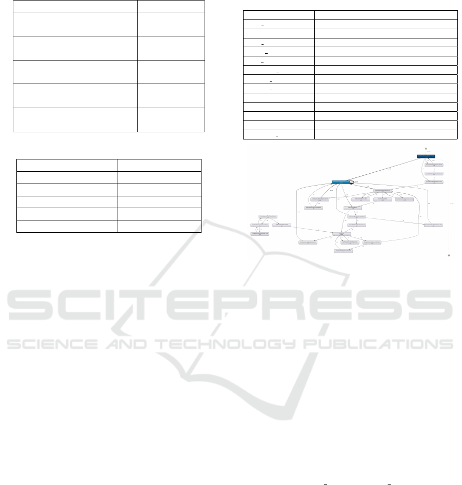
Table 1: Most common activities in the process.

Activity Name Occurrences

Invoice Approval Task

Conﬁrmation of receipt

114811

Invoice Approval Task

Invoice Approval

89579

Error

19651

Invoice Rejection Handling

Invoice Rejection AP WFT

7748

Error

Technical Error

7205

Table 2: Distribution of activities per case.

Number of activities Number of cases

1 activity 143858

2 activities 23400

3 activities 9132

4 activities 2473

5 or more activities 4121

There are 23 different activities that can happen

during the invoice approval process. Some examples

are: InvoiceApprovalTask - Conﬁrmation of receipt;

InvoiceApprovalTask - Invoice approval; InvoiceAp-

provalTask - Budget variance; InvoiceRejectionHan-

dling - Invoice Rejection AP WFT; ManageBuyerRe-

jection - Missing Goods Receipt; Error - Error; Error

- Technical Error; and RequestforAdditionalInforma-

tion - Request for Information. If a case is only com-

posed by activities starting with ”InvoiceApproval...”

it is considered that the case follows the ”happy” path.

In total, there are 182.984 cases and 270.921 ac-

tivities (23 unique ones), which means that, on av-

erage, a case is composed by 1,48 activities. Table

1 summarizes the most common activities and their

number of occurrences. The average time of a case

is 7,7 days, while the median time is 2,9 days. This

means that there are some outliers that have a high

inﬂuence on the average time.

It is also important to analyze the distribution of

activities in cases, in order to know what kind of pro-

cess is being analyzed. Table 2 shows this distribu-

tion. Most of the main variants in the process are com-

posed of one single activity, which proves that cases

are likely to be short. This information is useful to

explain the insights found in section 4.1 and the con-

ﬁguration chosen to build a transition system in 5.1.

4.1 Data Analysis

In this section a deeper analysis about the data is per-

formed. Firstly, in section 4.1.1, the preprocessing

Table 3: Columns of the ﬁnal table and their meanings after

preprocessing.

Column Explanation

case id Identiﬁer of a case

activity Activity of the process

start time Starting time of the activity

ﬁnish time Finish time of the activity

user id User that did the activity

company code Place to where the item was shipped

vendor id Identiﬁer of a vendor

vendor summarized Attribute to reduce the number of vendors

currency Currency of the invoice

price Price of the line item

status Final status of the invoice

approved 1 if approved, 0 if cancelled or reversed

purchase order 1 if related to a purchase order, 0 otherwise

Figure 3: Initial image shown by Disco.

needed to train the models and to understand the pro-

cess is explained. Then, in section 4.1.2, the insights

obtained using process mining are presented. Disco

was used to do so.

4.1.1 Preprocessing

Data were provided in four CSV ﬁles: general info,

invoice, invoice item and status. These ﬁles were

loaded in a MySQL database. A new table with all

the connections between the initial ﬁles was created

using MySQL scripts. Table 3 shows the columns

(with their meaning) of this new table, it also includes

some (not real for conﬁdentiality reasons) examples.

The ﬁrst 5 columns are related to the process, while

the rest are attributes related to the case. All columns

except activity, start time and ﬁnish time are repeated

so that the data can be correctly interpreted by the ap-

plication when they are loaded in the program.

4.1.2 Process Mining Analysis

The tool used for this task was Disco. The table cre-

ated in the previous section was exported into a CSV

ﬁle and used as input for these tools.

When the data is loaded, an image of the process

like the one of ﬁgure 3. This is just showing some of

the connections that exist, and it can be observed that

it is a complex process.

MODELSWARD 2019 - 7th International Conference on Model-Driven Engineering and Software Development

476

The initial approach consisted on analysing which

activities where the slowest ones. In order to not

be inﬂuenced by outliers, the median was taken, in-

stead of the average. The slowest activities are: Price

Variance, Invoice Approval Group task and Estimated

price. The last one does not occur too often, but the

other two do.

After this initial analysis, the cases were split in

two groups: those that followed the ”happy” path and

those that did not. In the case of the ﬁrst ones, they

wanted to analyse where the bottlenecks were. It was

found that the main bottlenecks are in the same activ-

ities mentioned above, but also in the connection be-

tween some activities: Invoice Approval and Budget

Variance; and Invoice Approval and Conﬁrmation of

Receipt. In theory, the cases should move between ac-

tivities without time delay, so this was a non expected

ﬁnding.

Then, the analysis of the cases that did not follow

the ”happy” path was done. These cases were those

that contained, at least, one of the following activi-

ties (deﬁned by experts): Approve Block Removal,

Decide to Wait for Answer or Withdraw, Invoice Re-

jection Handling, Manage Buyer Rejection, Manual

Approver Entry, Manual Approver Selection, Request

for Additional Information, Select Approver and Wait

for Credit. These cases were 6% of the total (11.655).

5 Results

5.1 Transition System

As explained in 3.1, to build a transition system some

choices need to be made. There are three different ab-

stractions and the chosen values were the following.

• Maximal Horizon: To choose this value it is im-

portant to know that there are in total more than

180.000 cases, and a lot of them follow different

paths. The key point is to ﬁnd a good balance

between enough information kept and an efﬁcient

system. The following values were analysed: 1

(current activity), 2, 3 and 4. In the case of 1, there

were 23 states, as many as different activities. In

the case of 2, there were 218 different states, in the

case of 3, 785 and in the case of 4, 1.617. The best

results were achieved with horizon 1, so it was the

chosen one.

• Filter: Activities were not ﬁltered, since there are

not many in total (23) and all of them are consid-

ered important.

• Sequence, Bag or Set: After analysing the cases

and talking to experts from the ﬁnance department

Table 4: Recarray containing the transition system.

ID Case ID State 1

State 1

...

State 23

0 1384571... 1 0 150 ... 240

1 3189485... 1 120313 1450 ... 120

182573 EI01-17... 1 0 150000 ... 1000

the decision was to take into account the order of

the activities in every case, since the ﬁnal outcome

is inﬂuenced by this fact. This abstraction does

not inﬂuence the transition system because the we

use horizon 1.

This transition system only focuses on past activ-

ities since the intention is to use it for prediction in

real time, when future activities are not available.

One of the main challenges of building a transi-

tion system having more than 180.000 cases and 23

different states is to build it fast and for it to occupy

the least memory possible. For every case that is in a

state, the elapsed time until the case got to that state

is kept, as well as the remaining time since the case

enters that state until the case is ﬁnished. This data,

together with the attributes related to the line items,

are used later on in the prediction phase. There is

a column that contains if the case went through that

state or not (0 and 1 as values) and the other two to

keep the times elapsed and remaining (in seconds).

To avoid having a bigger transition system, only

cases with 15 activities or less were taken into ac-

count. There are only 310 cases that have more than

15 activities, and most of them were classiﬁed as not

relevant cases by experts from the ﬁnance department.

The transition system was stored in a numpy re-

carray

, due to its high speed when iterating through

it. This kind of array is known because its columns

can have names. In this case, apart from the columns

related to the states we have a column that contains

the case IDs.

As explained above, the outcome is an array with

two dimensions, so it can be seen as a matrix whose

rows represent the cases, and the columns are: the

case ID (string), the states and the elapsed and re-

maining times for the states. When a case has been

through a state, there is a 1 in the corresponding cell,

and the cells related to the elapsed and remaining

times contain the time in seconds. Table 4 shows an

extract of how the recarray looks.

https://docs.scipy.org/doc/numpy/reference/generated/

numpy.recarray.html

An Approach for Workﬂow Improvement based on Outcome and Time Remaining Prediction

477

5.2 Final Status Prediction

The objective is to predict the outcome of each invoice

(Approved, Reversed, Cancelled) in real time. One

new prediction will be made every time an activity

occurs (the case moves from one state to another in

the transition system). Vendor, company code, price,

if the invoice is related to a purchase order or not,

currency and time elapsed were taken into account in

order to do the prediction.

As the data is so imbalanced (91% of the cases

are approved, 6% cancelled, and 3% reversed) and,

from the business and ﬂow point of view, cancelled

and reversed cases are really similar, both of them are

uniﬁed under the class NotApproved. This way, the

problem is less imbalanced and the classiﬁcation has

to be done only between two classes, which should

help improving the performance.

The objective is to predict the outcome in each ac-

tivity with the intention of improving it as the case

progresses since the state in which it is will be consid-

ered. To take into account the state of the transition

system for the prediction, one model will be built in

each state, taking as training data only the cases that

have been through that state. This model, apart from

the initial attributes, will also take into account the

elapsed time of the cases. This is the way Data Min-

ing and Process Mining are combined in this project.

In order to train the models, 80% of the data is

used in cross validation (to ﬁnd the best conﬁgura-

tion of each model) and the 20% remaining is used to

test which model is the best. Cross validation is set

up with 5 splits and it is stratiﬁed, this means each

split has the same distribution of Approved and No-

tApproved as the initial dataset.

The following techniques are compared: SVM,

random forest, K-NN and Naive Bayes. Different

conﬁgurations of the models are compared using the

ROC curve, since data is imbalanced and using ac-

curacy would not be a correct approach (classifying

everything as approved would return a 91% of accu-

racy). The ﬁnal comparison between the best conﬁg-

urations of the models is done using the ROC Curve,

F1 score, recall and precision, taking as the main class

the NotApproved cases (Cancelled and Rejected).

As more than 90% of the cases are ’Approved’, an

up-sampling and down-sampling technique was ap-

plied with the intention of improving the balance of

the dataset. The function used was SMOTETTomek

(Batista et al., 2003), which consists in a mix of down-

sampling the major classes and up-sampling the mi-

nor classes.

A summary of the different attributes available for

each case and activity is shown:

• Vendor id: There are 4.766 different vendors, each

of them with an ID. More than 2.000 appear only

3 times or less.

• Vendor id summarised: To reduce the number

of vendors some IDs were modiﬁed. Vendors

whose invoices have always been approved were

assigned ID 1, those whose invoices have al-

ways been reversed were assigned ID 2; and those

whose invoices have always been been cancelled

were assigned ID 3. All the other vendors were

assigned their own IDs. The number of vendors

was reduced from 4.700s to 1.600s.

• Company code: It identiﬁes to which part of the

company the ordered item belongs to.

• Price of the line item.

• Currency: There are more than 10 different cur-

rencies, and it is considered an important variable

at the moment of approving or not approving a

line item (together with the price).

• Purchase order related: Identiﬁes items related to

a Purchase Order Number (1) or unrelated (0).

• Time elapsed until the case reached the current

state.

Vendor id, vendor summarised, company code,

currency are categorical attributes, and it is neces-

sary to apply one hot encoding (Vasudev, 2017). It

consists on converting categorical attributes into bi-

nary variables. It is important to remark that due to

this, the number of attributes increases exponentially,

from 7-8 to almost 5000, which slows down the train-

ing of the models. This is why vendor summarised

was created, with the intention of reducing the ﬁnal

number of attributes (by more than 3000). Vendor

summarised was used instead of vendor id because

it improved the results and the execution time.

5.2.1 Comparison

This section compares different conﬁgurations of the

algorithm, sampling and not sampling training data.

The ones with the best Area under the ROC curve

(AUROC) are kept. A model is trained individually

in every state of the transition system, and sampling

is applied individually to the data from each state.

The performance between these two approaches

(without and with sampling) is compared using the

area under the ROC curve. The thresholds used are

set up manually, from 0 to 1 every 0,01, there be-

ing in total 101 thresholds. As mentioned before,

each state has its own model, but to compare two ap-

proaches it is easier if the results of all the states are

summarised into one single result. Knowing that to

MODELSWARD 2019 - 7th International Conference on Model-Driven Engineering and Software Development

478

Table 5: Comparison for ﬁnal status prediction using the

best conﬁgurations from several models.

Algorithm Conﬁguration AUROC

Random Forest

Not sampling

100 estimators

Class weight ”None”

0,5935

LinearSVC

Not sampling

Loss function ”Hinge”

Class weigth ”None

0,5032

K-NN

Sampling

50 neighbours

Manhattan Distance

0,5690

Gaussian

Naive Bayes

Not sampling

Default Conﬁguration

0,5032

Table 6: Comparison between Random Forest and K-NN.

Method

Best

Threshold

F1 Score Precision Recall AUROC

Random Forest 0,09 30,92 22,45 50,94 0,6869

K-NN 0,47 23,06 15,64 56,40 0,6461

generate a ROC curve the True Positive Rate (TPR)

and False Positive Rate (FPR) with different thresh-

olds are needed, their values obtained in each state

are averaged taking into account the number of cases

that are part of each state (weighted average).

Initially, in every state of the transition system, the

TPR and FPR are calculated for each different thresh-

old taking into account the number of cases that are in

the state. Then, for each threshold, the TPR and FPR

are obtained by adding the values speciﬁed in the pre-

vious step. These values can be used to draw a ROC

curve and obtain the area under it. The models with

their best conﬁgurations are shown in table 5.

The best conﬁgurations of the best algorithms pre-

sented (the bold ones) are compared using the testing

data (20% not used before). The Naive Bayes and

LinearSVC approaches are discarded because of their

low AUROC value. This leaves two different algo-

rithms to compare: Random Forest and K-NN.

Random Forest has a better AUROC, but in this

section other metrics such as the F1 score, the pre-

cision and the recall are also compared. To compare

the F1 score, the precision and the recall it is neces-

sary to choose a threshold. The threshold is chosen

using the Youden’s index (Ruopp et al., 2008). This

comparison is made in table 6. The conclusion is that

Random Forest performs better since it has a better F1

score (even though the recall is lower than in K-NN).

5.3 Time Remaining Prediction

This section presents the different approaches that

were followed to predict the time left of a case un-

til completion. The methods tested were regression

methods: bagging, boosting, random forest, MLR,

Table 7: Comparison for time remaining prediction using

the best conﬁgurations from several models.

Method Conﬁguration

MSE

Hours ˆ2

MAE

Hours ˆ2

Exec.

Time (sec.)

Average - 103.324 171,2 27

Random

Forest

50 estimators 118.929 172,6 10.257

K-NN

50 neighbours

Manhattan Distance

106.267 174,0 290

Boosting

Gradient Method

Learning Rate 0,08

50 estimators

98.227 166,0 1.348

Bagging

Default

Conﬁguration

122.226 174,7 1.079

LASSO and K-NN, as speciﬁed in 3.3. To test the

different conﬁgurations, cross validation was used, as

recommended in (Sharma et al., 2013).

The time elapsed and the time remaining are kept

in every state of the transition system. This makes

possible predicting remaining time of a case in every

state. The time is kept in seconds. The attributes used

for this section are the same as the ones in section 5.2.

In order to train the models, 80% of the data is

used in cross validation (to ﬁnd the best conﬁguration

of each model) and the 20% remaining is used to test

which model is the best. Cross validation is set up

with 5 splits.

5.3.1 Comparison

To compare the different conﬁgurations of each model

the Mean Squared Error (MSE) and Mean Absolute

Error (MAE) are the used metrics. To better under-

stand the results obtained, the Mean Squared Error

and the Mean Absolute Error are converted into hours.

The procedure followed to obtain the MSE and the

MAE of a method is the following. For each state,

cross validation is applied (5 splits). In each itera-

tion, 4 splits are used for training and one for valida-

tion. The MSE and MAE are stored for each case that

is validated, then, the average of both metrics is ob-

tained, and it is used to compare the different conﬁgu-

rations. The best conﬁgurations for the tested models

are presented in table 7. MLR and LASSO are not

shown since the results obtained were extremely bad.

The best conﬁgurations of the best algorithms pre-

sented (in bold) are compared using the testing data

(20% not used before). These algorithms are: av-

erage, K-NN and Gradient Boosting. In table 8, it

can be observed that the best results are obtained with

Gradient Boosting, regarding MSE and MAE.

The time of training might be important since the

model needs to be updated when new cases are over.

In this case, the fastest methods are average and K-

NN, but Gradient is also fast.

It can be observed that, on average, the models

are around 160 hours off in each prediction. Cases

An Approach for Workﬂow Improvement based on Outcome and Time Remaining Prediction

479

Table 8: Performance analysis for time remaining predic-

tion.

Method MSE Hours

MAE Hours

Execution Time

(in seconds)

Average 98.498,91 171,34 7

K-NN 96.481,01 166,89 79

Gradient Boosting 85.460,92 159,48 381

last, on average, 184,8 hours. The median duration of

a case is 70,2 hours. This means that the predictions

are bad given the median and average duration, but it

is important to take into consideration how much the

duration of a case can vary and the number of activ-

ities of a case. Usually, a short case is composed of

one activity, while longer cases can be composed of

3 or more activities. The short ones, easy to predict,

go just through one state; while the others go through

more states and are harder to predict. This means that

the long cases, which go through more states, are pre-

dicted more times, and they are more likely to be miss

predicted (since they are so far from normal values).

This leads to the ”high” errors shown above. There

are over 10.000 cases that last 30 days or more, and

they appear, on average, in 3 states. These cases will

have more weight than short cases on the MSE and

MAE shown above.

6 CONCLUSIONS AND FUTURE

WORK

In this paper we presented an approach to have in-

sights about a business process. The approach is

mainly divided into three parts: 1) a transition system;

2) a ﬁnal status prediction; and 3) a time remaining

prediction. For that, Process Mining and Data Mining

techniques were used. Several data mining algorithms

were built over the different states of a transition sys-

tem. This way, the path that a case followed was taken

into account.

To validate our approach, we used a case study

from a ﬁnancial department with real life data. The

transition system allowed to take into account the path

that a case followed by just using the cases that are

in the same state to train the data mining model (for

status and time remaining prediction).

The case study used to test classiﬁcation al-

gorithms had two main problems: 1) imbalanced

dataset, with more than 90% of the cases being ap-

proved, and 2) some cases have similar attributes and

similar paths, but they have different ﬁnal status. For

this scenario, as explained in Section 5, to predict the

ﬁnal status of a case Random Forest was the algorithm

with the best performance.

Regarding the time remaining prediction, interest-

ing results were achieved with different algorithms.

The poor performance of the linear models proved

that there is no linear relation between the attributes

and the time until completion. The best results were

achieved with Gradient Boosting.

REFERENCES

Aalst, van der, W., Schonenberg, M., and Song, M. (2011).

Time prediction based on process mining. Information

Systems, 36(2):450–475.

Antonio, L., Seabra, R. M., Biagio, P., Ricardo, R., and

Christian, C. (2017). A comparison of advanced

regression techniques for predicting ship co2 emis-

sions. Quality and Reliability Engineering Interna-

tional, 33(6):1281–1292.

Batista, G. E. A. P. A., Bazzan, A. L. C., and Monard, M. C.

(2003). Balancing training data for automated anno-

tation of keywords: a case study. In WOB.

Ruopp, M. D., Perkins, N. J., Whitcomb, B. W., and Schis-

terman, E. F. (2008). Youden index and optimal cut-

point estimated from observations affected by a lower

limit of detection. Biometrical journal. Biometrische

Zeitschrift, 50 3:419–30.

Sharma, S., Agrawal, J., and Sharma, S. (2013). Article:

Classiﬁcation through machine learning technique:

C4.5 algorithm based on various entropies. Interna-

tional Journal of Computer Applications, 82(16):28–

32. Full text available.

van der Aalst, W. M. P., Rubin, V., Verbeek, H. M. W.,

van Dongen, B. F., Kindler, E., and G

unther, C. W.

(2008). Process mining: a two-step approach to bal-

ance between underﬁtting and overﬁtting. Software &

Systems Modeling, 9(1):87.

van Dongen, B. F., Crooy, R. A., and van der Aalst, W.

M. P. (2008). Cycle time prediction: When will this

case ﬁnally be ﬁnished? In Meersman, R. and Tari,

Z., editors, On the Move to Meaningful Internet Sys-

tems: OTM 2008, pages 319–336, Berlin, Heidelberg.

Springer Berlin Heidelberg.

Vasudev, R. (2017). What is one hot encod-

ing? why and when do you have to use it?

https://hackernoon.com/what-is-one-hot-encoding-

why-and-when-do-you-have-to-use-it-e3c6186d008f.

Accessed: [11/07/2018].

Zeng, S., Melville, P., A. Lang, C., M. Boier-Martin, I.,

and Murphy, C. (2008). Using predictive analysis to

improve invoice-to-cash collection. pages 1043–1050.

MODELSWARD 2019 - 7th International Conference on Model-Driven Engineering and Software Development

480