Coordinated Image- and Feature-space Visualization for Interactive

Magnetic Resonance Spectroscopy Imaging Data Analysis

Muhammad Jawad, Vladimir Molchanov and Lars Linsen

Westf

alische Wilhelms-Universit

at M

unster, Germany

Keywords:

Multidimensional Data Visualization, Medical Visualization, Coordinated Views, Spectral Imaging Analysis.

Abstract:

Magnetic Resonance Spectroscopy Imaging (MRSI) is a medical imaging method that measures per voxel a

spectrum of signal intensities. It allows for the analysis of chemical compositions within the scanned tissue,

which is particularly useful for tumor classiﬁcation and measuring its inﬁltration of healthy tissue. Common

analysis approaches consider one metabolite concentration at a time to produce intensity maps in the image

space, which does not consider all relevant information at hand. We propose a system that uses coordinated

views between image-space visualizations and visual representations of the spectral (or feature) space. Co-

ordinated interaction allows for analyzing both aspects and relating the analysis results back to the other for

further investigations. We demonstrate how our system can be used to analyze brain tumors.

1 INTRODUCTION

Magnetic Resonance Spectroscopy Imaging (MRSI)

is an in-vivo medical imaging method for measuring

chemical compositions of scanned tissues. The com-

positions in the form of metabolite concentrations can

be computed from spectral information of chemical

resonance (Gujar et al., 2005). While T1- or T2-

weighted Magnetic Resonance Imaging (MRI) data

allows for the detection of tumors and to determine

their shape, MRSI provides additional information on

their metabolic activity. Such information, on the one

hand, allows for a classiﬁcation of the tumor with re-

spect to its malignancy (from benign to malignant),

and, on the other hand, for an investigation, whether

the tumor has already started inﬁltrating surrounding

“healthy” tissue (Burnet et al., 2004).

The metabolic information is extracted from the

spectrum for each voxel of the MRSI data in a pre-

processing step, see Section 3.2. Afterwards, the in-

formation at hand is the metabolic concentration of all

extracted metabolites per voxel. The set of metabo-

lites form a multidimensional space, which we refer

to as the spectral or feature space. Each voxel is re-

ﬂected by a point in this multidimensional space. On

the other hand, the voxels have a spatial arrangement

in the image space.

Common analysis tools for MRSI data in clini-

cal settings visualize the spatial distribution of indi-

vidual metabolite concentrations using color mapping

of an image slice. Thus, only a single metabolite is

investigated at a time. Therefore, a lot of informa-

tion is being neglected and the interplay of metabo-

lites concentrations cannot be analyzed. We propose

a novel tool that integrates all information at hand

for a comprehensive analysis of MRSI data. Our ap-

proach is based on coordinated views of visualiza-

tion in image and feature space. For image space,

we also use slice-based visualizations, as they avoid

occlusion and it is common to only scan a few slices

in MRSI. MRSI visualizations are overlaid with MR

images and combined with automatic MRI segmen-

tation results. For feature space, multidimensional

data visualization methods are used. Given the image

segmentation result, the multidimensional data are la-

beled accordingly and we apply interaction methods

to separate the labeled classes. Using star-coordinates

encoding, the separations can be related back to the

individual dimension, basically allowing for conclu-

sions, which metabolite concentration allow for class

separation. The methodology is detailed in Section 4.

In Section 5, we apply our methods to a scenario

for MRSI data analysis to investigate brain tumors.

In 2012, WHO reported 256,213 brain cancer cases,

of which 189,382 deaths have been recorded (Board,

PDQ Adult Treatment Editorial, 2018). We show how

our coordinated views allow for analyzing the brain

tumor’s chemical composition as well as the inﬁltra-

tion of surrounding tissue that when based on MRI

data may be classiﬁed as non-tumor region.

118

Jawad, M., Molchanov, V. and Linsen, L.

Coordinated Image- and Feature-space Visualization for Interactive Magnetic Resonance Spectroscopy Imaging Data Analysis.

DOI: 10.5220/0007571801180128

In Proceedings of the 14th International Joint Conference on Computer Vision, Imaging and Computer Graphics Theory and Applications (VISIGRAPP 2019), pages 118-128

ISBN: 978-989-758-354-4

2 RELATED WORK

Nunes et al. (Nunes et al., 2014a) provided a sur-

vey of existing methods for analyzing MRSI data.

They conclude that no approach exists that analyzes

all metabolic information. They report that MRSI

data visualization packages provided with commer-

cial scanners such as SyngoMR and SpectroView

only provide color mapping of individual metabolic

concentrations (or a ratio of metabolic concentra-

tions) in image space. Other tools such as Java-based

Magnetic Resonance User Interface (jMRUI) (Stefan

et al., 2009) and Spectroscopic Imaging Visualization

and Computing (SIVIC) (Crane et al., 2013) that are

also widely used in clinical practice provide a simi-

larly restricted functionality.

Raschke et al. (Raschke et al., 2014) proposed

an approach to differentiate between tumor and non-

tumor regions by showing the relation of concentra-

tions of two selected metabolites in a scatterplot. By

plotting the regression line, they identiﬁed abnormal

regions by data points that are far from the line. Sim-

ilarly, Rowland et al. (Rowland et al., 2013) use scat-

terplots to inspect three different pairs of metabolites

tumor analysis. These procedures only target selected

metabolites, which are chosen a priori.

An approach to exploit the metabolic informa-

tion better was presented by Maudsley et al. (Maud-

sley et al., 2006). They developed the Metabolite

Imaging and Data Analysis System (MIDAS) for

MRSI pre-processing and visualization. Users can

view histograms of metabolites, but relations between

metabolites cannot be studied. Feng et al. (Feng

et al., 2010) presented the Scaled Data Driven Sphere

(SDDS) technique, where information of multiple

metabolite concentrations is combined in a glyph-

based visualization using mappings to color and size.

Obviously, the amount of dimensions that can be

mapped is limited. They overlay the images with

the glyphs and link them to parallel coordinate plots.

Users can make selections in the parallel coordinate

plot and observe respective spatial regions in the im-

age space. As a follow-up of their survey, Nunes et

al. (Nunes et al., 2014b) presented a system that cou-

ples the existing systems ComVis (Matkovic et al.,

2008) and MITK (Wolf et al., 2004). They use scatter-

plot, histogram, and parallel coordinate plot visualiza-

tions for analyzing the metabolic features space. The

visualizations provide linked interaction to image-

space representations such that brushing on metabolic

data triggers highlighting in image space.

We build upon the idea of using coordinated inter-

actions in feature and image space, but enhance the

functionality signiﬁcantly: We incorporate segmen-

tation results, provide means to separate the labeled

data in feature space, allow for a comparative visual-

ization of classes, and provide a single tool that inte-

grates all information and allows for fully coordinated

interaction in both directions.

3 BACKGROUND

In this section, we provide background on the imaging

method, describe the executed pre-processing steps,

describe the data at hand after imaging and pre-

processing, and the driving questions.

3.1 Imaging

MRSI is an in-vivo medical imaging method, where

per voxel a whole spectrum of intensities is recorded.

While MRI only measures water intensities per voxel,

MRSI measures intensities at different radio frequen-

cies. Most commonly

H MRSI is used, where the

signal of hydrogen protons (

H) in different chemi-

cals is measured in the form of intensity peaks. As

this measurement is performed for different frequen-

cies, different chemicals can be detected within each

voxel. The intensity peaks within the frequency spec-

trum are quantiﬁed as parts per million (ppm).

Measuring entire spectra in MRSI comes at the

expense of much lower spatial resolution when com-

pared to MRI. Using 1.5T or 3T scanners yields voxel

sizes of about 10mm × 10mm × 8mm (Nunes et al.,

2014a; McKnight et al., 2001). 7T scanners yield-

ing higher resolutions are barely used in clinical prac-

tice due to high costs (Scheenen et al., 2008). Typ-

ically, MR images are taken (using T1 or T2 relax-

ation) in addition to MRS images within the same ses-

sion. The MR images provide anatomical information

at a higher resolution.

3.2 Pre-processing

The main goal of the pre-processing step is to quan-

tify the various chemicals, referred to as metabo-

lites, within each voxel from the respective intensity

spectrum. MRSI is not yet standardized (e.g., us-

ing a DICOM format), but there is open source and

proprietary software available for pre-processing and

metabolite quantiﬁcation like LCModel (Provencher,

1993), jMRUI (Stefan et al., 2009), and Totally Au-

tomatic Robust Quantitation in NMR (TARQUIN)

(Reynolds et al., 2006).

Common pre-processing steps provided by the

tools are eddy current compensation, offset correc-

tion, noise ﬁltering, zero ﬁlling, residual water sup-

Coordinated Image- and Feature-space Visualization for Interactive Magnetic Resonance Spectroscopy Imaging Data Analysis

119

pression, and phase and base line correction. These

steps are executed in the measured time domain or

in the frequency domain after performing a Fourier

transform. Signal strength in time domain indicates

the metabolites’ concentration, while the area under

the metabolite curve is used to compute the concen-

tration in frequency domain. The computed values are

similar when measurements with high signal-to-noise

ratio are provided (Vanhamme et al., 2001). For the

actual metabolite concentration, mathematical mod-

els are used and ﬁtted to the measured data. Different

tools use different ﬁtting approaches.

For the pre-processing of our data, we used TAR-

QUIN, which is an open-source GUI-based soft-

ware for in-vivo spectroscopy data pre-processing and

quantiﬁcation. It operates in time domain and uses a

non-negative least-squares method for model ﬁtting to

compute the metabolite concentrations. We incorpo-

rate TARQUIN in our data preparation step due to free

availability, friendly user interface, automatic quan-

tiﬁcation, support for multi-voxel spectroscopy, and

being able to process various ﬁle formats and to ex-

port the results in various formats (Reynolds et al.,

2006; Wilson et al., 2011).

3.3 Data

The data we use in this paper for our applica-

tion scenario was acquired using an

H MRSI tech-

nology on a 3T Siemens scanner (TR/TE/ﬂip =

1700ms/135ms/90

◦

). Two MRSI series are taken,

each having a 160mm × 160mm × 1mm ﬁeld of view.

In addition, an MRI volume is captured and regis-

tered with the MRSI volume. The MRI volume is

224mm×256mm×144mm with 1 mm slice thickness.

We clip the MRI volume to the MRSI volume. The

resolution of the MRI volume is much higher such

that each MRSI voxel stretches over 10mm × 10mm ×

12mm MRI voxels. The data are courtesy of Miriam

Bopp and Christopher Nimsky from the University

Hospital Marburg, Germany. We used TARQUIN for

MRSI pre-processing and metabolite quantiﬁcation.

The quantiﬁcation process resulted in 33 metabolites

that are listed in Table 1.

After metabolite quantiﬁcation, we can summa-

rize the available data as two slabs of MRSI voxels

with registered MRI voxels. For each MRSI voxel,

we have computed concentrations of 33 metabolites,

leading to a 33-dimensional feature space, where each

point in the feature space represents the chemical

composition of one voxel. In addition, we know for

each MRSI voxel, which are the matching MRI vox-

els (single intensity values). In the following, we will

propose methods for visualization in image space and

Table 1: Metabolites delivered by a quantiﬁcation from

brain MRSI data using TARQUIN.

No. Name No. Name No. Name

1 Ala 12 Lip09 23 PC

2 Asp 13 Lip13a 24 PCr

3 Cr 14 Lip13b 25 Scyllo

4 GABA 15 Lip20 26 Tau

5 GPC 16 MM09 27 TNAA

6 Glc 17 MM12 28 TCho

7 Gln 18 MM14 29 TCr

8 Glth 19 MM17 30 Glx

9 Glu 20 MM20 31 TLM09

10 Ins 21 NAA 32 TLM13

11 Lac 22 NAAG 33 TLM20

feature space, where coordinated interaction within

the linked views is used to analyze the MRSI data.

3.4 Driving Questions

MRSI data are mainly acquired to analyze tumors. In

our application scenario, we look into brain tumors.

The ﬁrst driving question is the tumor classiﬁcation,

i.e., one would want to ﬁnds out what type of tumor

it is and how its malignancy is rated. To do so, one

should analyze the MRSI voxels belonging to the tu-

mor. The question one would like to answer with

MRSI measurements is then: What are the chemi-

cal compositions of the tumor? The second important

question is whether the tissue surrounding the tumor

is already inﬁltrated by the tumor. MRSI allows for a

more detailed analysis of the surrounding tissue. The

question to be answered is then: How do the chemical

composition in areas surrounding the tumor compare

to those of the tumor and to those of healthy tissue?

Finally, one may want to see whether tumors in other

regions occur, i.e., one would ask: Are there other ar-

eas that have a similar chemical composition as the

tumor?

4 METHODOLOGY

4.1 Image Space Visualization

In order to analyze image regions such as tumors or

surrounding tissue, one would need to be able to vi-

sually inspect those regions and interactively select

them. We support this using a slice-based viewer,

which we implemented using the VTK (Schroeder

et al., 2006) and ITK (Johnson et al., 2013) libraries.

Within the slice, we have two visualization layers.

The ﬁrst layer represents the MRI volume. It pro-

IVAPP 2019 - 10th International Conference on Information Visualization Theory and Applications

120

vides the anatomical context for the MRSI data analy-

sis, see Figure 1. A greyscale luminance color map is

used, as this is a common standard in MRI visualiza-

tion. The second layer represents the MRSI volume.

Here, individual voxels can be selected interactively

by brushing on the image regions. Selected voxels

are highlighted by color, see Figure 7(left).

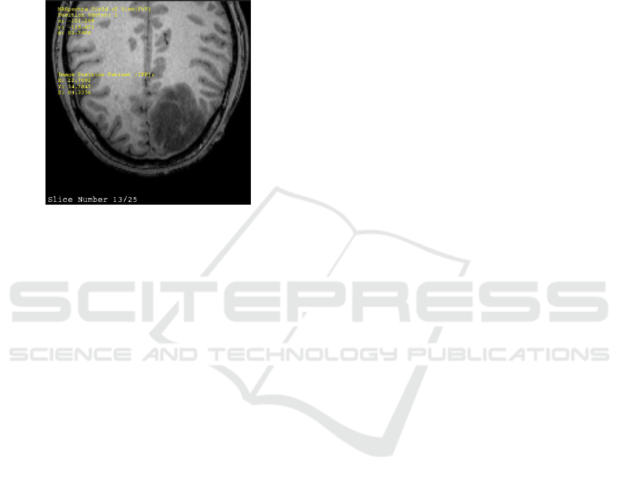
Figure 1: Anatomical context in slice-based image-space

MRI visualization.

In addition to manual selection of MRSI voxels

based on visual inspection, we also support an au-

tomatic image segmentation method. The automatic

image segmentation predeﬁnes regions for quick se-

lection and region analysis. The automatic segmenta-

tion method partitions the MR image. A large range

of algorithms exist each having certain advantages

and drawbacks. For the data at hand, the best re-

sults in our tests were obtained by the Multiplicative

Intrinsic Component Optimization (MICO) (Li et al.,

2014) segmentation method for auto characterization

of various tissues in brain MRI. MICO could handle

MRI with low signal-to-noise ratio that is due to mag-

netic ﬁeld disturbance and patient movement during

the scanning process. MICO performs well in bias

ﬁeld estimation and in discarding intensity inhomo-

geneity.

If we impose the MR image segmentation result

on the MRSI voxels, we have to deal with partial vol-

ume effects, as one MRSI voxel corresponds to many

MRI voxels, which may be classiﬁed differently. We

propose to use a visual encoding that conveys the par-

tial volume effect. Instead of simply color-coding

the MRSI voxel by the color for the dominant class

among the MRI voxels, we render square glyphs that

are ﬁlled with different colors, where the color por-

tions reﬂect the percentages how often the MRI vox-

els are assigned to the respective class. Figure 2

shows a respective slice-based visualization, where

the segmentation result is shown in the MRSI layer

overlaying the MRI layer. The mixture of colors indi-

cate the uncertainty of the anatomical region segmen-

tation at the MRSI resolution. In the image, we show

the glyphs for each of the dominant class, i.e., the ﬁve

columns (from left to right) show MRSI voxels, where

the respective MRI voxels have primarily been classi-

ﬁed as background, cerebrospinal ﬂuid (CSF), tumor,

gray matter, and white matter, respectively. The col-

ors used for the respective classes are shown above

the images. Results are shown for both MRSI slabs.

4.2 Feature Space Visualization

The feature-space visualization problem is that of a

multidimensional data visualization problem, where

dimensionality is in the range of tens, while the num-

ber of data points is in the range of hundreds. Hence,

we need an approach that scales sufﬁciently well in

both aspects. Moreover, the tasks require us to ob-

serve patterns such as clusters of data points, i.e., sets

of data points that are close to each other and different

from other data points. Many multidimensional data

visualization approaches exist and we refer to a recent

survey for their descriptions (Liu et al., 2017). They

can be distinguished by the performed data transfor-

mations, by the visual encodings, and by their map-

pings to visual interfaces. Point-based visual encod-

ings scale well in the number of data points and al-

low for an intuitive detection of clusters. Among

them, projection-based dimensionality reduction ap-

proaches use data transformations to a visual inter-

face supporting the handling of high dimensionality.

Linear projections have the advantage over non-linear

projections that the resulting plots can be easily re-

lated back to the original dimensions by the means

of star coordinates. Thus, we propose to use star-

coordinates plots (Kandogan, 2000) to visualize the

feature space.

A projection from an n-dimensional feature space

to a 2D visual space is obtained by a projection ma-

trix of dimensions 2 × n, where each of the n columns

represent the tip of the n star-coordinates axes. The

default set-up is to locate the tips equidistantly on

the unit circle, see Figure 3. The tips can be moved

to change the projection matrix, which allows for an

interactive multidimensional data space analysis sup-

porting the detection of trends, clusters, outliers, and

correlations (Teoh and Ma, 2003).

When assuming an image-space segmentation of

the voxels as described in the preceding section, each

voxel is assigned to a class. Hence, we are dealing

with labeled multidimensional data. A common task

in the visual analysis of labeled multidimensional data

is to ﬁnd a projected view with a good separation of

the classes. This is also of our concern, as we want

Coordinated Image- and Feature-space Visualization for Interactive Magnetic Resonance Spectroscopy Imaging Data Analysis

121

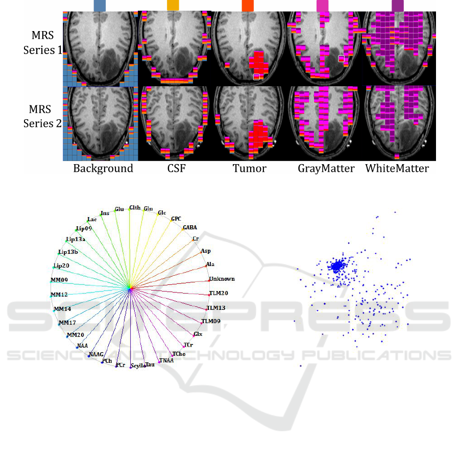
Figure 2: MRI segmentation visualized at MRSI resolution using glyphs with color ratios that reﬂect class distribution of each

voxel.

Figure 3: Default star-coordinates conﬁguration (left) and respective projection of 33-dimensional feature space to a 2D visual

space. Each dimension represents a metabolite concentration, each point corresponds to a MRSI voxel.

to separate tumor from healthy tissues. Molchanov et

al. (Molchanov and Linsen, 2014) proposed an ap-

proach for intuitive interactive class separation in lin-

early projected views. We adopt their idea for our pur-

poses. The idea is to use a control point for each class,

e.g., being the classes’ medians. Classes can then be

separated by dragging control points apart. Since the

visual representation is restricted to linear projections,

the position to which the control points are dragged

can, in general, not be exactly obtained in a linear

projection. Molchanov et al. proposed to use a least-

squares approach to ﬁnd the best match to the desired

interaction. Using this idea, the user just needs to

move the control points of the classes in an intuitive

manner, where the number of classes is usually low

(ﬁve in the case of brain imaging data), instead of

interacting with all star-coordinates axes, which be-

comes tedious for larger number of dimensions (33 in

our application scenario). Figure 4 illustrates this by

showing the star-coordinates conﬁguration to the left

and the linear projection of the labeled multidimen-

sional data to the right, where the control points that

can be interactively moved are the ones with a black

frame. Since the visualization would be too cluttered

when overlaying the two views, we decided to show

them in a juxtaposed manner. Further argumentation

for juxtaposed views of star coordinates is provided

by Molchanov and Linsen (Molchanov and Linsen,

2018).

Since the points in our projected view represent

MRSI voxels, while the image segmentation is per-

formed on the higher-resolution MR image, we have

partial volume effects as discussed in the previous

section. The uncertainty of the labeling result shall

also be conveyed in our projected view. For example,

if some points are identiﬁed as outliers of a cluster,

one should be able to reason if the labeling of the re-

spective voxel is uncertain or not. If it was uncertain,

the outlyingness may be due to a wrong labeling deci-

sion. To visually convey the labeling uncertainty, the

IVAPP 2019 - 10th International Conference on Information Visualization Theory and Applications

122

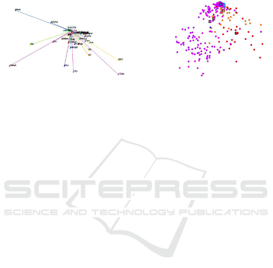
Figure 4: Interactive visual analysis of labeled multidimensional data: star-coordinates conﬁguration (left) and respective

projected view (right) obtained by interacting with control points (black frames) of the classes induced by image segmentation.

probabilities of each point belonging to each class la-

bel shall be represented. Since the probabilities sum

up to one, they are well represented by a pie chart, i.e.,

each point in the projected view is displayed by a pie

chart. Figure 5 shows a projected view with labeling

uncertainty conveyed by pie charts.

While interacting with the control points in the

projected view, the star-coordinates axes are up-

dated accordingly. Hence, when separating classes

in the projected view, one can observe in the star-

coordinates view, which axes are mainly responsible

for the separation, i.e., which axes are the ones that

allow for such a separation. The dimensions that are

associated with these axes are subject to further in-

vestigations, as one of our tasks was to detect the

metabolic compositions of tumors and surrounding

tissues. For selected metabolites, we use different sta-

tistical plots supporting different analysis steps.

If we are interested in investigating the metabolic

compositions of two classes for selected metabolites,

we use juxtaposed box plots to show the statistical in-

formation of the metabolic concentrations of all vox-

els that were assigned to each class. The box plots

convey the median, the interquartile range, as well as

minimum and maximum, see Figure 12.

If we are interested in investigating the interplay

of two metabolites, we can analyze their correlation

using a 2D scatterplot. Scatterplots are most effec-

tive in showing correlation and detecting outliers, see

Figure 6(right). Correlation analysis is supported

by computing and displaying a regression line. In

case more than two metabolites shall be analyzed si-

multaneously, parallel coordinate plots allow for a

good correlation analysis and scale better than scat-

terplot matrices in the number of dimensions, see Fig-

ure 7(right).

4.3 Coordinated Interaction in Image

and Feature Space

The interactive visual analysis becomes effective

when using coordinated interaction of the image- and

feature-space views. In the image space, one can

brush the MRSI voxels in the slice-based visualiza-

tion and group them accordingly. Hence, interactive

labeling is supported. Of course, one can also use the

labeling that is implied by the MRI segmentation (in-

cluding the uncertainty visualization). The resulting

labeling is transferred to the projected feature-space

visualization by using the same colors in both visu-

alizations, see image-space visualization in Figure 2

and respective projected feature-space visualization

in Figures 4 and 5. This coordinated interaction al-

lows for investigating whether image segments form

coherent clusters in feature space, which dimensions

of the feature space allow for a separation of the clus-

ters, and whether there are some outliers. Of course,

the same holds true when using the statistical plots

as a coordinated feature-space view. Figure 6 shows

a brushing in image space and investigation of the

selection in a scatterplot visualization of two (previ-

ously selected) dimensions, while Figure 7 shows a

brushing in image space and investigation of the se-

lection in a parallel coordinate plot of seven (previ-

ously selected) dimensions.

The coordinated interaction of image and feature

space is bidirectional. Thus, the user may also brush

in the feature space, e.g., by selecting a group of

points in the feature space that form a cluster, and

observe the spatial distribution of the selection in the

image space. Again, one can use any of the feature-

space visualizations or a combination thereof. For ex-

ample, in Figure 8, the four voxels to the left are cho-

sen (voxels having low concentration of TNAA rela-

tive to TCho and TCr) in the bar chart and the respec-

tive highlighting in the image space convey that these

Coordinated Image- and Feature-space Visualization for Interactive Magnetic Resonance Spectroscopy Imaging Data Analysis

123

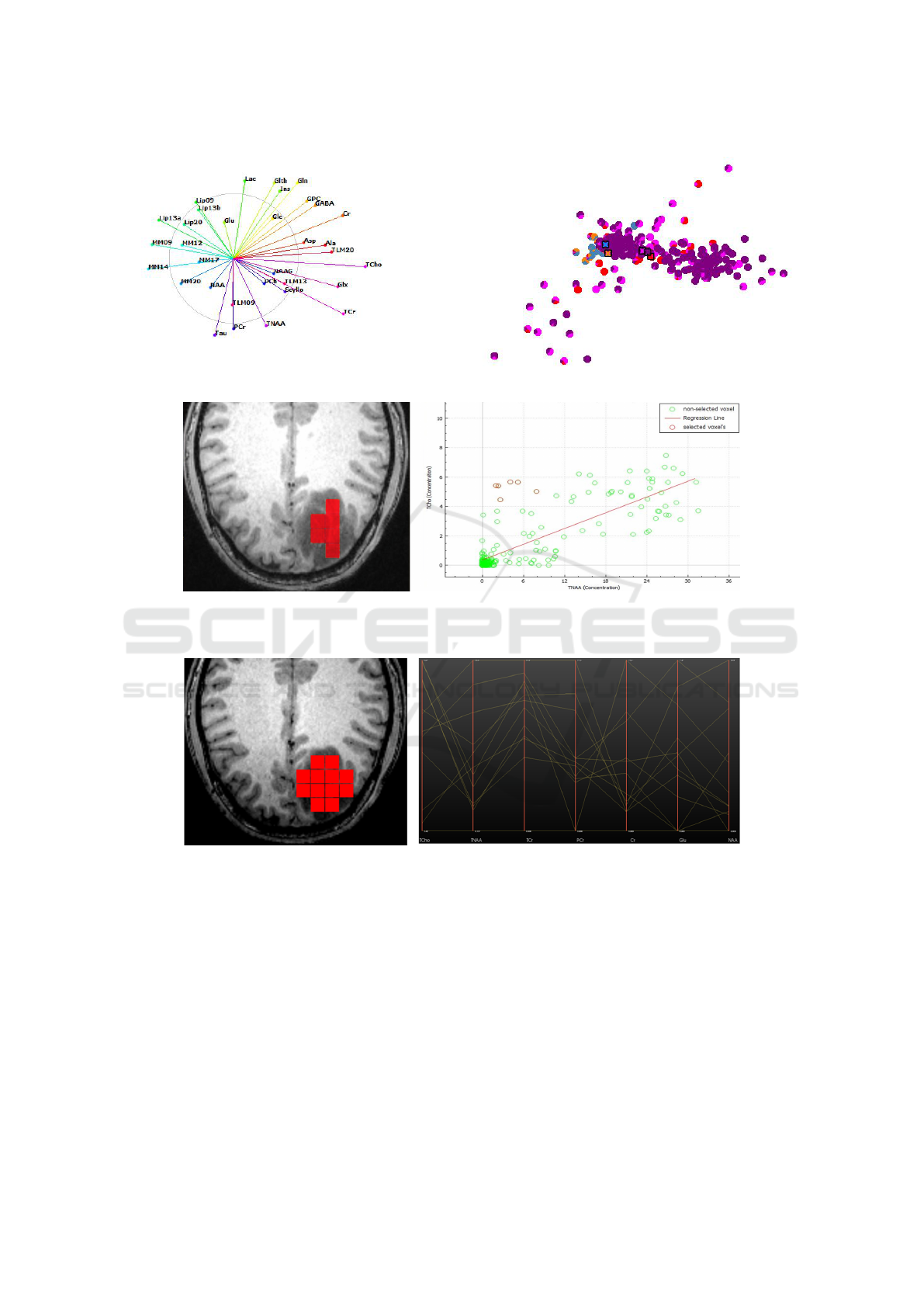
Figure 5: Pie-chart representation of uncertainty for projected points.

Figure 6: Correlation analysis of the metabolites TCho and TNAA in a scatterplot (right) and detection of outliers. Voxels

corresponding to the interactively selected outliers are shown in the image-space visualization (left), which conveys their

relation to the tumor.

Figure 7: (left) Interactive selection of MRSI voxels in image space and (right) linked view for correlation analysis of seven

selected metabolites (TCho, TNAA, TCr, PCr, Cr, Glu, and NAA) using parallel coordinate plot for the selected voxels.

voxels belong to the tumor region.

We also support a heatmap visualization as com-

monly used when observing the spatial distribution of

individual metabolite concentrations. The user may

select a single metabolite or a combination of metabo-

lites. Figure 9 shows heatmaps of TCho and TNAA

concentrations and In Figure 10, a heatmap of the log-

arithm of the ratio of TCho/TNAA is shown.

The full potential of our system is reached by us-

ing coordinated interaction in both ways simultane-

ously. For example, one can select the tumor voxels

in the image space, can investigate the respective set

of points in feature space possibly forming a cluster,

detect further points that fall into the cluster, select

those further points, and observe their spatial distri-

bution. These newly selected voxels may be voxels

surrounding the tumor, in case the tumor has already

inﬁltrated surrounding regions, or may be voxels that

form a region elsewhere, in case there is a second tu-

mor.

IVAPP 2019 - 10th International Conference on Information Visualization Theory and Applications

124

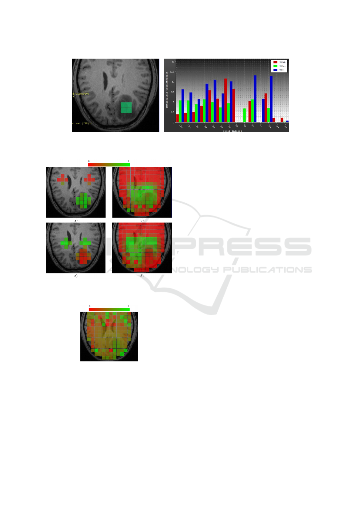
Figure 8: Concentration of three selected metabolites shown side by side in the bar chart (right). Four voxels with low

concentration of TNAA relative to TCho and TCr are selected by brushing. The coordinated image-space view (left) highlights

the selected voxels, which form the core of the tumor.

Figure 9: Heatmaps of TCho (top) and TNAA concentration

(bottom) for all brain voxels (right) and selected regions of

interest (left).

Figure 10: Heatmap of ratio of TCho/TNAA concentrations

(in logarithmic scaling).

5 RESULT AND DISCUSSION

In our application scenario, we applied the developed

methods of Section 4 to the data acquired from a 26-

year old male patient with a brain tumor. MRSI and

MRI head scans were obtained as described in Sec-

tion 3.3. We preprocessed the data as described in

Section 3.2. Then, we ﬁrst investigated the projected

feature space using the default star-coordinates lay-

out as in Figure 3. We observe no obvious clus-

ters in the projected space. Thus, we next applied

an automatic segmentation of the MR image and im-

posed the segmentation onto the MRSI voxels using

our uncertainty-aware visualization in Figure 2. The

extracted segments represent grey matter, white mat-

ter, CSF, the tumor, and background. This segmen-

tation implies a labeling as shown in Figure 4, where

the colors match with the ones in Figure 2. We ap-

plied the interactive technique to separate the classes

in feature space using the interaction with the classes’

control points. In particular, we applied it to separate

the tumor class (red) from the other classes. We ob-

serve that certain dimensions of our 33-dimensional

feature space are affected strongly by this interactive

optimization. Hence, the respective metabolites may

be the ones that distinguish tumor from the other seg-

ments. In Figure 4, we see that the axes labeled NAA,

Glu, TNAA, PCr, TCr, TCho, and GPC are longest.

These metabolites are candidates for further investi-

gations. In Figure 6, we select TNAA and TCho con-

centrations, which had the longest axes in Figure 4

and plot all voxels in a scatterplot. We select a group

of outliers (red) with high TCho and low TNAA con-

centrations and observe that these form the core of

the tumor region. Please note that by just looking at

one of the two metabolites the voxels would have not

been outliers. In Figure 9, we use heatmaps to in-

vestigate the spatial distributions of TCho and TNAA

concentrations, respectively. When looking at the en-

tire brain region (right image column), it is hard to

detect structures. However, when selecting regions of

interest such as a white matter region and the tumor

region, we can spot the differences (left image col-

umn). The two columns apply the red-to-green color

map to the minimum-to-maximum range of selected

voxels only. In Figure 10, a heatmap of the logarithm

of the ratio of the two metabolites is shown.

Coordinated Image- and Feature-space Visualization for Interactive Magnetic Resonance Spectroscopy Imaging Data Analysis

125

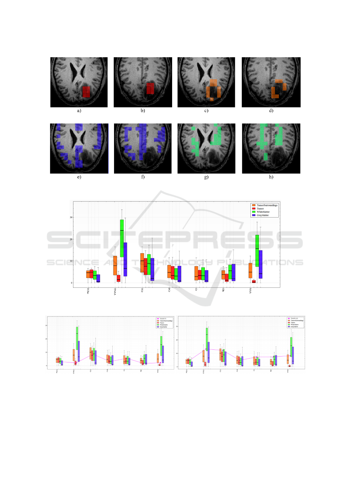
Figure 11: Interactive labeling of voxels within both MRSI slabs representing tumor (red), voxels in the vicinity of the tumor

(orange), grey matter (blue), and white matter (green).

Figure 12: Juxtaposed box plots to compare class statistics for selected classes (voxels labeled as white matter, grey matter,

tumor, and surrounding tumor) and selected metabolites.

Figure 13: Metabolite concentration of voxels 73 (left) and 123 (right) in vicinity of the tumor selected in Figure 11 in

comparison to the concentrations of the tumor, white matter, and grey matter classes.

When investigating the projected feature space in

Figure 4, we observe that the classes are actually not

well separated. We further investigate the pie chart

visualization of the labeling result, see Figure 5 to

observe quite a few voxels that are rather uncertain

with respect to the automatic labeling, which may

be due to the partial volume effect. Also, when se-

lecting all voxels that contain parts of the tumor as

IVAPP 2019 - 10th International Conference on Information Visualization Theory and Applications

126

in Figure 7, the distribution of values in the parallel

coordinate plot appear rather diverse. Thus, we de-

cided to manually select regions of low-uncertainty

voxels and create new labels, see Figure 11. Fig-

ure 12 shows the juxtaposed box plots of the four se-

lected voxel groups. We observe that the tumor re-

gion (red) is quite different from the other regions

in NAA and TNAA concentrations, where TNAA is

the sum of NAA and NAAG. We also observe that

the voxels surrounding the tumor (orange) behave like

gray/white matter voxels rather than tumor voxels for

these metabolites, which makes us believe that these

voxels are not yet inﬁltrated by the tumor. How-

ever, this may not be true for individual voxels of that

group. Since the tumor size and shape of its bound-

ary is important for diagnosis and treatment, we se-

lected individual voxels at the border of the tumor

and investigated the metabolite concentrations and in-

dividually compared their metabolite concentrations

to those of tumor as well as white and grey matter.

Figure 13 shows such a comparison for the voxels

labeled 73 and 123 in Figure 11. These two voxels

showed high uncertainties in the automatic segmenta-

tion result. We can observe in Figure 13 that voxel 73

matches well the tumor class, while voxel 123 does

not. Hence, we conclude that the tumor may already

have inﬁltrated the area at voxel 73, while it may have

not yet done so for voxel 123.

We invited two MRSI experts with many years

of experience of acquiring and analyzing MRSI data

to our lab to show them our tool on a large multi-

touch display. The visual encodings were mostly in-

tuitive to them and they were quickly able to suggest

interactive analysis steps themselves. Only the pro-

jected view needed some explanations, but the intu-

itive interaction with the control points made them

adopt the concept quickly. They also quickly brought

in their expertise into the analytical workﬂow by ex-

cluding some metabolites that they knew would not

be important for the given tasks such as lipids and

macromolecules and by interpreting correctly combi-

nations such as TNAA being a combination of NAA

and NAAG. In the session, we jointly looked into

the metabolic composition of voxels in the vicinity

of the tumors as documented above. To test the re-

producibility of the analysis, it would be desirable to

test our tool with a large number of experts on a large

number of data sets. We hope that we can conduct

such a study in future work, but acknowledge that it

will be challenging to recruit a large number of ex-

perts.

6 CONCLUSIONS AND FUTURE

WORK

We presented a comprehensive tool for the analysis

of MRSI data and applied it to brain tumor investi-

gations. Using coordinated views of image and fea-

ture space visualizations, effective analysis steps can

be performed that allow for a comprehensive inves-

tigation of all data facets. We showed how relevant

metabolites can be identiﬁed and how image regions

can be detected and compared. In this paper, we fo-

cused on the analysis of a tumor region. Future direc-

tions include the analysis of different tumor types, for

which MRSI information from many patient shall be

combined, eventually leading to a cohort analyses.

ACKNOWLEDGEMENTS

This work was supported in part by DFG grant MO

3050/2-1.

REFERENCES

Board, PDQ Adult Treatment Editorial (2018). Adult cen-

tral nervous system tumors treatment PDQ

. In PDQ

Cancer Information Summaries. National Cancer In-

stitute (US).

Burnet, N. G., Thomas, S. J., Burton, K. E., and Jefferies,

S. J. (2004). Deﬁning the tumour and target volumes

for radiotherapy. Cancer Imaging, 4(2):153–161.

Crane, J. C., Olson, M. P., and Nelson, S. J. (2013). SIVIC:

open-source, standards-based software for DICOM

MR spectroscopy workﬂows. Journal of Biomedical

Imaging, 2013:12.

Feng, D., Kwock, L., Lee, Y., and Taylor II, R. M. (2010).

Linked exploratory visualizations for uncertain MR

spectroscopy data. In Park, J., Hao, M. C., Wong,

P. C., and Chen, C., editors, Visualization and Data

Analysis 2010. SPIE.

Gujar, S. K., Maheshwari, S., Bj

orkman-Burtscher, I.,

and Sundgren, P. C. (2005). Magnetic reso-

nance spectroscopy. Journal of neuro-ophthalmology,

25(3):217–226.

Johnson, H. J., McCormick, M., Ib

nez, L., and Consor-

tium, T. I. S. (2013). The ITK Software Guide. Kit-

ware, Inc., third edition.

Kandogan, E. (2000). Star coordinates: A multi-

dimensional visualization technique with uniform

treatment of dimensions. In In Proceedings of

the IEEE Information Visualization Symposium, Late

Breaking Hot Topics, pages 9–12.

Li, C., Gore, J. C., and Davatzikos, C. (2014). Multi-

plicative Intrinsic Component Optimization (MICO)

for MRI bias ﬁeld estimation and tissue segmentation.

Magnetic resonance imaging, 32(7):913–923.

Coordinated Image- and Feature-space Visualization for Interactive Magnetic Resonance Spectroscopy Imaging Data Analysis

127

Liu, S., Maljovec, D., Wang, B., Bremer, P., and Pascucci,

V. (2017). Visualizing high-dimensional data: Ad-

vances in the past decade. IEEE Transactions on Vi-

sualization & Computer Graphics, 23(3):1249–1268.

Matkovic, K., Freiler, W., Gracanin, D., and Hauser, H.

(2008). ComVis: A coordinated multiple views sys-

tem for prototyping new visualization technology. In

2008 12th International Conference Information Visu-

alisation, pages 215–220. IEEE.

Maudsley, A., Darkazanli, A., Alger, J., Hall, L., Schuff, N.,

Studholme, C., Yu, Y., Ebel, A., Frew, A., Goldgof,

D., et al. (2006). Comprehensive processing, display

and analysis for in vivo MR spectroscopic imaging.

NMR in Biomedicine, 19(4):492–503.

McKnight, T. R., Noworolski, S. M., Vigneron, D. B., and

Nelson, S. J. (2001). An automated technique for

the quantitative assessment of 3D-MRSI data from

patients with glioma. Journal of Magnetic Reso-

nance Imaging: An Ofﬁcial Journal of the Interna-

tional Society for Magnetic Resonance in Medicine,

13(2):167–177.

Molchanov, V. and Linsen, L. (2014). Interactive design

of multidimensional data projection layout. In N.

Elmqvist, M. Hlawitschka, and J. Kennedy, editors,

EuroVis - Short Papers. The Eurographics Associa-

tion.

Molchanov, V. and Linsen, L. (2018). Shape-preserving star

coordinates. IEEE Transactions on Visualization &

Computer Graphics, pre-print.

Nunes, M., Laruelo, A., Ken, S., Laprie, A., and B

uhler,

K. (2014a). A survey on visualizing magnetic reso-

nance spectroscopy data. In Proceedings of the 4th

Eurographics Workshop on Visual Computing for Bi-

ology and Medicine, pages 21–30. Eurographics As-

sociation.

Nunes, M., Rowland, B., Schlachter, M., Ken, S., Matkovic,

K., Laprie, A., and B

uhler, K. (2014b). An integrated

visual analysis system for fusing MR spectroscopy

and multi-modal radiology imaging. In Visual Analyt-

ics Science and Technology (VAST), 2014 IEEE Con-

ference on, pages 53–62. IEEE.

Provencher, S. W. (1993). Estimation of metabolite concen-

trations from localized in vivo proton NMR spectra.

Magnetic resonance in medicine, 30(6):672–679.

Raschke, F., Jones, T., Barrick, T., and Howe, F. (2014). De-

lineation of gliomas using radial metabolite indexing.

NMR in Biomedicine, 27(9):1053–1062.

Reynolds, G., Wilson, M., Peet, A., and Arvanitis, T.

(2006). An algorithm for the automated quantitation

of metabolites in in vitro NMR signals. Magnetic res-

onance in medicine, 56(6):1211–1219.

Rowland, B., Deviers, A., Ken, S., Laruelo, A., Ferrand,

R., Simon, L., and Laprie, A. (2013). Beyond the

metabolic map: an alternative perspective on MRSI

data. ESMRMB 2013, 30th Annual Scientiﬁc Meeting,

page 270.

Scheenen, T. W., Heerschap, A., and Klomp, D. W. (2008).

Towards

H-MRSI of the human brain at 7T with

slice-selective adiabatic refocusing pulses. Mag-

netic Resonance Materials in Physics, Biology and

Medicine, 21(1-2):95–101.

Schroeder, W., Martin, K., Lorensen, B., Avila, Sobierajski,

L., Avila, R., and Law, C. (2006). The Visualization

Toolkit. Kitware, Inc., fourth edition.

Stefan, D., Di Cesare, F., Andrasescu, A., Popa, E.,

Lazariev, A., Vescovo, E., Strbak, O., Williams, S.,

Starcuk, Z., Cabanas, M., et al. (2009). Quantita-

tion of magnetic resonance spectroscopy signals: the

jMRUI software package. Measurement Science and

Technology, 20(10):104035.

Teoh, S. T. and Ma, K.-L. (2003). StarClass: Interactive

visual classiﬁcation using star coordinates. In SDM,

pages 178–185. SIAM.

Vanhamme, L., Sundin, T., Hecke, P. V., and Huffel,

S. V. (2001). MR spectroscopy quantitation: a re-

view of time-domain methods. NMR in Biomedicine,

14(4):233–246.

Wilson, M., Reynolds, G., Kauppinen, R. A., Arvanitis,

T. N., and Peet, A. C. (2011). A constrained least-

squares approach to the automated quantitation of in

vivo

H magnetic resonance spectroscopy data. Mag-

netic resonance in medicine, 65(1):1–12.

Wolf, I., Vetter, M., Wegner, I., Nolden, M., Bottger, T.,

Hastenteufel, M., Schobinger, M., Kunert, T., and

Meinzer, H.-P. (2004). The Medical Imaging interac-

tion ToolKit MITK: A toolkit facilitating the creation

of interactive software by extending VTK and ITK.

volume 5367, pages 5367 – 5367 – 12.

IVAPP 2019 - 10th International Conference on Information Visualization Theory and Applications

128