A Uniﬁed Curvature-driven Approach for Weathering and Hydraulic

Erosion Simulation on Triangular Meshes

era Skorkovsk

a, Ivana Kolingerov

a and Petr Van

cek

Department of Computer Science and Engineering, Faculty of Applied Sciences,

University of West Bohemia, Univerzitn

ı 8, Plze

n, Czech Republic

Keywords:

Erosion Simulation, Weathering, Hydraulic Erosion, Mesh Deformation.

Abstract:

Erosion simulation is an important problem in the ﬁeld of computer graphics. The most prominent erosion

processes in nature are weathering and hydraulic erosion. Many methods address these problems but they are

mostly based on height ﬁelds or volumetric data. Height ﬁelds do not allow for the simulation of complex

fully 3D scenes while the volumetric data have high memory requirements. We propose a uniﬁed approach

for weathering and hydraulic erosion working directly on triangular meshes which simpliﬁes the use of the

method in wide range of scenarios. We take into account the observation that the speed of erosion in nature

is affected by the local shape of the eroded object. We use estimation of mean curvature to drive the speed of

erosion, which results in visually plausible simulation of erosion processes. We demonstrate the results of the

method on both artiﬁcial 3D models and on real data.

1 INTRODUCTION

Erosion is mainly perceived as the process that

changes the look of the landscape over the years but it

also affects smaller individual objects. In the ﬁeld of

computer graphics and animation, it is mainly used as

a means to create realistic looking landscapes and to

simulate aging effects. Many methods have addressed

the simulation of different types of erosion processes,

however, there are still many open problems.

Most of the existing solutions work either with

volumetric data or with height ﬁelds. The height

ﬁelds are very convenient for erosion simulation as

they can be easily used to store large-scale terrains.

The simplicity of the data structure also allows for

very fast methods but it cannot be used to capture

fully 3D scenes containing concave features and com-

plex topology. On the other hand, the volumetric data

structures can represent any object but it is usually at

the cost of higher memory requirements and slower

speed of the simulation.

As triangular meshes are by far the most com-

monly used object representations in computer graph-

ics, it is reasonable to design methods using this struc-

ture. The main advantage of triangular meshes in re-

lation to erosion simulation is their adaptivity and the

possibility to model complex concave features. The

triangular mesh data structure allows to model an ob-

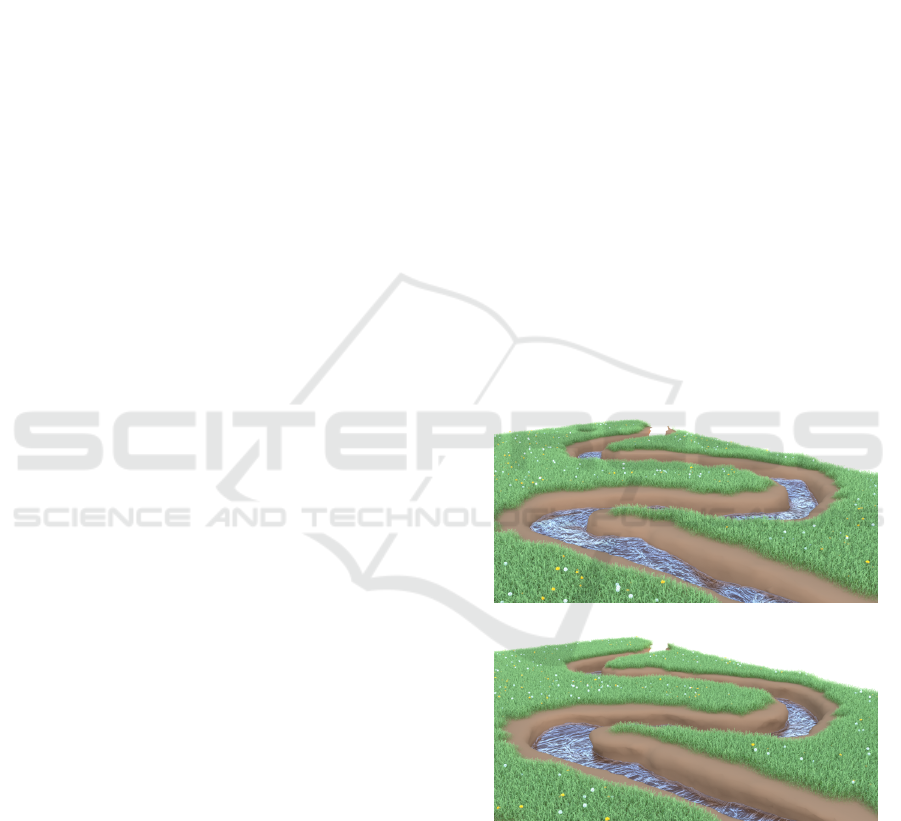
Figure 1: Running water creates undercuts on the river

banks; front view. Original model (top) and the scene af-

ter 200 iterations (bottom) of hydraulic erosion simulation.

ject adaptively with varying density of vertices based

on the complexity of the object, leading to lower

memory requirements of the scene when compared

to the volumetric approaches, while it keeps the abil-

ity to model fully 3D scenes with complex features.

However, the use of triangular data structures intro-

duces other challenges. It may be more difﬁcult to es-

122

Skorkovská, V., Kolingerová, I. and Van

cek, P.

A Uniﬁed Curvature-driven Approach for Weathering and Hydraulic Erosion Simulation on Triangular Meshes.

DOI: 10.5220/0007566401220133

In Proceedings of the 14th International Joint Conference on Computer Vision, Imaging and Computer Graphics Theory and Applications (VISIGRAPP 2019), pages 122-133

ISBN: 978-989-758-354-4

timate the object properties such as curvature on irreg-

ular data structures. Also, when the triangular mesh

is being deformed during the simulation, it has to be

deformed in such a manner that does not damage its

integrity.

We propose a fast method that is working directly

on triangular meshes and uses curvature estimation

to drive the speed of erosion to simulate visually

plausible erosion scenarios without using complex

physically-based erosion function. The idea to use the

curvature of the object to control the speed of erosion

is supported by the observation of the erosion pro-

cesses in real life. The areas with high mean curvature

are more exposed to natural inﬂuences and are eroded

at a faster rate, while the areas with zero or negative

curvature are more protected and are eroded at much

slower rate. We focus our efforts on spheroidal weath-

ering and hydraulic erosion processes as these have

the highest impact on the alteration of landscape ele-

ments over the years. Figure 1 shows a sample result

of our hydraulic erosion simulation. The ﬂuid rep-

resented by a particle system erodes the terrain and

undercuts the river banks creating distinct overhangs

especially in the river bends. The scene and erosion

simulation settings will be discussed in further detail

in Section 4.

To summarize, the main contributions of our paper

are:

• The simulation of spheroidal weathering and hy-

draulic erosion is performed directly on triangular

meshes.

• The simulation speed is driven by mean curvature

of the model which results in highly realistic re-

sults.

• The method represents a fast uniﬁed approach that

can be used to simulate both spheroidal weather-

ing and hydraulic erosion.

The paper is organized as follows: Section 2

presents the state-of-the-art methods in the ﬁeld of

erosion simulation. Section 3 describes the proposed

solution and Section 4 presents the results of the pro-

posed algorithm. Finally, Section 5 concludes the pa-

per.

2 RELATED WORK

Erosion is a process happening in nature by which

material such as sand and rocks is taken from its orig-

inal location, transported and deposited at another

location by means of water, wind or other natural

forces. Erosion is a long-term process that is usu-

ally studied in the context of terrain alteration where

it is the most noticeable. It can however also be ob-

served on smaller individual objects, such as rocks

and stones. The man-made objects, e.g., buildings,

roads or statues, are also affected by the erosion pro-

cesses. Weathering and hydraulic erosion are the two

types of erosion that have the highest impact on the

alteration of the landscape and as such are receiving

the highest attention.

Weathering is a process of breaking down rocks,

e.g., due to the contact with chemical substances, liv-

ing organisms or due to thermal changes. One of the

ﬁrst weathering approaches was presented by Mus-

grave et al. (Musgrave et al., 1989). They use a sim-

pliﬁed global erosion method to simulate weathering

on a fractal terrain stored as a height ﬁeld. Another

weathering approach was presented by Bene

s and Ar-

riaga (Bene

s and Arriaga, 2005) which was designed

to generate table mountains. Dorsey et al. (Dorsey

et al., 1999) presented a method for modeling and

rendering of weathered stones using a novel voxel

surface-aligned data structure called slab. This struc-

ture works as an intermediate between the stone and

the surrounding erosion factors and restrains the ero-

sion computation to the regions adjacent to the sur-

face. Jones et al. (Jones et al., 2010) presented

an algorithm for spheroidal and cavernous weather-

ing of rocks with concave surfaces. The algorithm

is built on a voxel grid and the erosion is calcu-

lated through the mean curvature estimation. Ty-

chonievich and Jones (Tychonievich and Jones, 2010)

proposed a weathering method using a tetrahedral

mesh data structure based on Delaunay deformable

models (DDM). They are able to generate visually

plausible results, however, the method is very com-

putationally expensive.

Hydraulic erosion is the erosion caused by still or

running water, but also the erosion caused by glaciers

or avalanches. It has the most noticeable impact on

the evolution of the landscape. The erosion caused

by rain can smooth the rocks and mountains while the

streams and rivers can cause the creation of river beds,

valleys or canyons. Hydraulic erosion methods can

be subdivided into two categories: physically inspired

methods and physically based methods.

The physically inspired methods take inspiration

in natural processes but do not try to simulate them

exactly. Their main purpose is to mimic the erosion

impacts with as little computational effort as possi-

ble, so that the results look good without the need to

simulate the exact physical erosion processes. Mus-

grave et al. (Musgrave et al., 1989) proposed a sim-

ple hydraulic erosion algorithm simulating rain ef-

fects on a terrain represented by a height ﬁeld. Chiba

et al. (Chiba et al., 1998) introduced a method based

A Uniﬁed Curvature-driven Approach for Weathering and Hydraulic Erosion Simulation on Triangular Meshes

123

on velocity ﬁelds of the water ﬂow. They use parti-

cles to approximate the water volume and the erosion

is evaluated when a particle collides with the terrain

stored as a height ﬁeld. Another height ﬁeld based hy-

draulic erosion method was presented by Bene

s and

Forsbach (Bene

s and Forsbach, 2002). They deﬁne

the hydraulic erosion through a process consisting of

four independent steps that can be repeatedly applied

to achieve the desired visual effect.

The physically based methods use hydrodynam-

ics in order to simulate the erosion processes more

exactly. However, even methods from this category

usually introduce some simpliﬁcations of the ﬂuid dy-

namics to speed up the simulation. Shallow water

simulation is a simpliﬁcation of Navier-Stokes equa-

tions for the ﬂuid dynamics that is often used for hy-

draulic erosion simulations. The shallow water model

does not allow overlaps such as breaking waves or

splashes but it is often sufﬁcient for erosion simula-

tions. It has been used to simulate hydraulic erosion,

e.g., by Bene

s (Bene

s, 2007) and Mei et al. (Mei et al.,

2007). A volumetric Eulerian approach is used by

Bene

s et al. (Bene

s et al., 2006) to create a fully 3D

simulation of hydraulic erosion. They represent both

the eroded object and the ﬂuid as a volumetric grid

and deﬁne the erosion using processes that alter the

state of the voxels of the scene. Wojtan et al. (Wo-

jtan et al., 2007) simulate corrosion and erosion of

solid objects stored as a level set and simulate the ero-

sion by advecting it inward and the deposition by ad-

vecting the level set outward. Other methods use La-

grangian approach and describe the ﬂuid using a par-

ticle system. Kri

stof et al. (Kri

stof et al., 2009) use

the particle-based Smoothed particle hydrodynamics

(SPH) to simulate erosion on terrains represented by

a height ﬁeld. They represent the water ﬂow with

the SPH particles that erode the terrain on collision.

Later, Crespin et al. (Crespin et al., 2014) extended

the method by representing the terrain as a 3D gener-

alized map (Lienhardt, 1994). A similar SPH-based

approach is used by Skorkovsk

a et al. (Skorkovsk

et al., 2015) to simulate hydraulic erosion on terrains

represented using triangular meshes.

The most recent methods focus on automated gen-

eration of large visually plausible landscapes. Cor-

donnier et al. (Cordonnier et al., 2016) presented a

method that combines tectonic uplift and hydraulic

erosion to achieve realistic-looking terrains. Later,

Cordonnier et al. (Cordonnier et al., 2017) extended

the method to take into account the vegetation and

simulate the mutual impact between the vegetation

and the terrain erosion during the evolution of the

landscape.

However, none of the aforementioned methods al-

lows for the simulation of erosion on small-scale but

complex fully 3D objects that would have sufﬁcient

quality and at the same time was not very computa-

tionally expensive.

3 PROPOSED SOLUTION

The proposed approach simulates erosion on objects

represented as triangular meshes and uses curvature

to control the degree of erosion at different parts of

the eroded object. The erosion is then simulated by

using vertex displacement in the direction given by

the vertex normal and the discrete Laplace-Beltrami

operator.

3.1 Curvature Estimation

Curvature is a surface property that describes how

bent a surface is at a given point. As the pro-

posed method works on discrete triangular meshes,

the curvature cannot be calculated exactly and has

to be estimated. There are many methods that can

be used to estimate curvature on triangular meshes;

for a thorough survey, the reader can refer to the

paper by V

sa et al. (V

sa et al., 2016). We

have used the curvature estimation as proposed by

Rusinkiewicz (Rusinkiewicz, 2004) due to its sim-

plicity and performance. However, any other curva-

ture estimator could be used in its place as we only

need the curvature to capture the rough shape of the

eroded object.

We use mean curvature H in our simulation as its

values correspond to the region types important for

erosion; the mean curvature is negative in concave re-

gions (valleys, gaps), zero in ﬂat areas and positive in

convex areas (hills). In the rest of the paper, we will

use the curvature color coding as depicted in Figure 2;

negative mean curvature is represented by blue color,

zero mean curvature by green color and positive mean

curvature by red color. As the curvature value is scale-

dependent, we downscale the curvature value interval

for each eroded object to ﬁt in the interval < −1,1 >.

To preserve the zero curvature areas, we ﬁnd value

H = max(|H

min

|,|H

max

|) (1)

and scale interval < −H,H > to interval < −1,1 >.

We do not alter the curvature values for scenes

where the curvature interval already ﬁts inside the in-

terval < −1,1 >, as it could cause problems in scenes

with almost no curvature.

GRAPP 2019 - 14th International Conference on Computer Graphics Theory and Applications

124

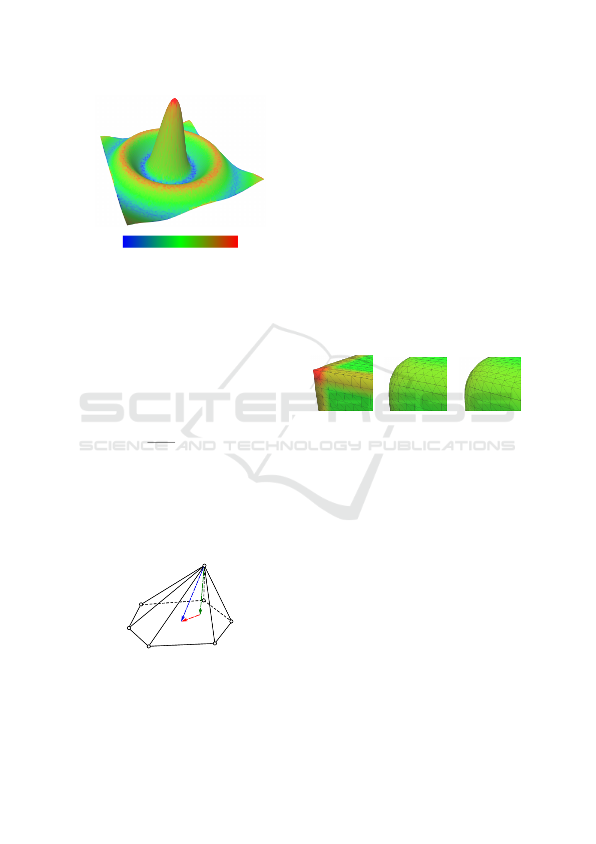
H<0

H=0

H>0

Figure 2: Curvature color coding. Negative mean curvature

is represented by blue color, zero mean curvature by green

color and positive mean curvature by red color.

3.2 Vertex Displacement

We use the mean curvature value to estimate the de-

sired magnitude of the erosion at the given vertex of

the mesh. To estimate the direction of the vertex dis-

placement, we use the vertex normal direction and the

discretization of the Laplace-Beltrami operator.

We use the uniform discretization of the Laplace-

Beltrami operator, which assigns a vector L

to each

vertex v

, such that

kN(i)k

∑

j∈N(i)

− v

), (2)

where N(i) is the set of vertices in the one-ring neigh-

borhood of the i-th vertex. The resulting vectors L

capture the tangential and normal offset of the vertex

from the average of its neighbors. In Figure 3, the

vector L

represents the uniform discretization of the

Laplace-Beltrami operator, the vector N

represents

the normal offset and the vector T

represents the tan-

gential offset.

Figure 3: Uniform discretization of Laplace-Beltrami oper-

ator.

As the uniform discretization of the Laplace-

Beltrami operator captures also the tangential offset,

it tends to regularize the distribution of the mesh ver-

tices. While this behavior can be undesirable in many

applications, it very well suits the needs of the erosion

simulation on triangular meshes in the regions of high

positive or negative curvature.

The vertex displacement can generally cause the

creation of small and badly shaped triangles if the di-

rection of the displacement is not chosen carefully.

The uniform discretization of the Laplace-Beltrami

operator and its ability to regularize the vertex dis-

tribution alleviates the problem and results in forma-

tion of more even triangles. Figure 4 captures the dif-

ference between results of the erosion simulation of

a cube when uniform discretization of the Laplace-

Beltrami operator and the opposite direction of the

vertex normal is used for the vertex displacement di-

rection. The left image shows the original mesh, the

center image shows the results of the simulation after

100 steps if the Laplace-Beltrami operator is used for

the vertex displacement direction, and the right im-

age shows the corresponding results if vertex normal

is used instead. It can be seen that the use of the uni-

form discretization of the Laplace-Beltrami operator

results in more regular and nicely shaped triangles.

Figure 4: Direction of vertex displacement. Original mesh

(left) after 100 simulation steps using the uniform dis-

cretization of the Laplace-Beltrami operator as displace-

ment direction (center) vs. the displacement in the opposite

direction of the vertex normal (right). Using curvature color

coding as described in Figure 2.

On the other hand, the displacement direction

based on the uniform discretization of the Laplace-

Beltrami operator can cause problematic artifacts in

the regions where the mean curvature is close to zero,

as the tangential shift can potentially damage the

mesh. For this reason, we use the direction of the uni-

form discretization of the Laplace-Beltrami operator

for weathering simulation where we erode only mesh

regions with positive mean curvature, while for the

hydraulic erosion simulation we use a combination of

the two aforementioned approaches.

3.3 Weathering

We simulate the weathering processes by displacing

the vertices in the areas with positive mean curvature

in the direction given by the uniform discretization

of the Laplace-Beltrami operator. The displacement

magnitude has to be chosen carefully in order to as-

sure that each step of the simulation ends with a valid

mesh. If the displacement is too big, inconsistencies

A Uniﬁed Curvature-driven Approach for Weathering and Hydraulic Erosion Simulation on Triangular Meshes

125

can be created in the mesh. Figure 5 demonstrates the

problem. If a small displacement step is applied, we

achieve the desired smoothing effect of erosion. If the

applied displacement is too big, the mesh can become

tangled as a result.

Figure 5: Small displacement step results in the desired

smoothing effect (left), while too big displacement can

damage the mesh (right).

To estimate a reasonable length of the displace-

ment, we take into account the average length of the

edges of the eroded mesh. The smaller the triangles of

the mesh, the shorter the displacement has to be in or-

der not to damage the mesh. We have experimentally

conﬁrmed that 1/10 of the average edge length is a

good threshold for the maximum displacement length

in a single step of the simulation. However, for some

highly irregular meshes this approach can still fail and

create inconsistencies in the highly detailed parts of

the meshes; in such a case we detect the problem by

ﬁnding the mesh self-intersections and we restart the

simulation with shorter displacements per step.

For each vertex v

we calculate the corresponding

displacement length d

as follows:

= H

avg

, (3)

where H

is the mean curvature at the vertex v

, e

avg

is the average edge length and x is the modiﬁer that

limits the maximum length of the displacement to be

1/x of the average edge length e

avg

. The position of

the vertex v

at the time step t is then calculated as

= v

t−1

+ d

, (4)

where L

represents the uniform discretization of the

Laplace-Beltrami operator at the vertex v

To enhance the erosion effect in the protruding re-

gions even more, we can use a power of the mean

curvature to calculate the erosion strength. As we still

want to keep the relation between the maximum ver-

tex displacement and the average edge length, the for-

mula for the calculation of the vertex displacement

length will become

= H

avg

,n ∈ R

≥1

, (5)

where n is the power modiﬁer of the mean curvature

value.

To validate the correctness of the weathering ef-

fect of the presented approach, we have applied the

erosion simulation to a cube model. Figure 6 shows

the original cube model and the model after 30, 100

and 200 steps. The power modiﬁer n was set to 1 for

this simulation. As can be seen in Figure 6, the algo-

rithm converts the cube to a sphere as expected.

3.4 Hydraulic Erosion

We propose a similar approach to simulate hydraulic

erosion. We use the particle-based simulation library

Flex by Nvidia (NVIDIA, 2014) to simulate the ﬂuid.

However, as we do not rely on any speciﬁc features of

the library, it could be easily exchanged for any other

particle-based ﬂuid simulation system.

To simulate the hydraulic erosion, we limit the

erosion processes to the regions of the mesh that are in

contact with the ﬂuid particles. For each ﬂuid particle

that collides with the mesh, we search for all the ver-

tices that are within the region of inﬂuence d

in f luence

of the particle. In our simulations, we set the region of

inﬂuence d

in f luence

to be equal to the average length of

the edge of the mesh, as it results in including most of

the vertices of the affected triangles while excluding

any vertices that are too distant from the ﬂuid parti-

cles. To speed up the search for the close vertices, we

use a simple auxiliary grid structure which stores the

information about the spatial subdivision of the mesh.

As we want to have a smooth transition between

the eroded and the still parts of the mesh, we calculate

the distance factor f

distance

of the vertex v

as follows:

distance

in f luence

− d

part

in f luence

, (6)

where d

part

is the distance between the vertex v

and

the closest particle. The distance factor f

distance

then used to inﬂuence the hydraulic erosion speed as

follows:

= v

t−1

+ d

distance

, (7)

where L

is the vertex displacement direction. For

the displacement direction, we use a combination

of the vertex normal and the uniform discretization

of the Laplace-Beltrami operator. For vertices with

mean curvature value of zero we use only the vertex

normal, while for the vertices with mean curvature of

min

or H

max

we use only the Laplace-Beltrami oper-

ator. For the remaining values, we use a linear inter-

polation of the vectors.

Unlike in the case of weathering, in hydraulic ero-

sion simulation we have to be able to erode all vertices

in the affected areas, regardless of their mean curva-

ture value. The stream of water erodes ﬂat areas as

GRAPP 2019 - 14th International Conference on Computer Graphics Theory and Applications

126

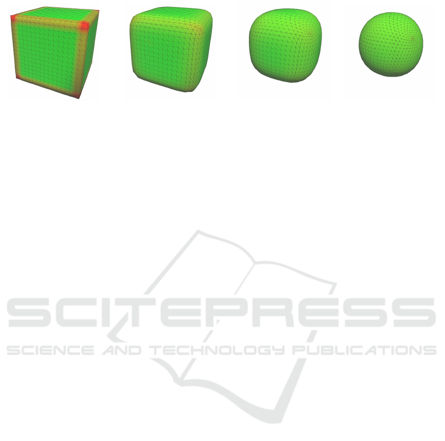
Figure 6: Validation of the weathering approach. From left to right: input cube model and the model after 30, 100 and 200

steps of the simulation. After 200 steps of the simulation, the input cube model has been eroded into a sphere. Using curvature

color coding as described in Figure 2.

well as gaps and protrusions, but the speed of the ero-

sion will differ. The strength of erosion in protruded

areas is the highest, followed by ﬂat areas and gaps.

To mimic this behavior, we use a different approach

for scaling the mean curvature. We scale the mean

curvature value interval < H

min

max

> to ﬁt in the

interval < 0,1 >. That way, the gaps are eroded more

slowly and protrusions faster, resulting in a visually

plausible simulation of erosion.

4 RESULTS

We have performed extensive testing to demonstrate

the visual quality of the results of our approach. This

section presents the results of our weathering and hy-

draulic erosion simulation algorithms.

4.1 Weathering

Figure 7 shows the results of the weathering method

applied on the model of the Stanford bunny (Levoy

et al., 2005). The ﬁgure demonstrates the inﬂuence

of the power modiﬁer n as introduced in Equation 5.

For the ﬁrst row of images, the power modiﬁer n = 1,

for the second row n = 2 and for the last row n = 3.

Each row then represents the state of the simulation

after increasing number of iterations. It can be seen

that the increase of power modiﬁer n results in slower

erosion rate in the ﬂatter regions.

The effect of the power modiﬁer n is the most

signiﬁcant on models with distinct protruded regions,

such as the hand model in Figure 8. The ﬁgure shows

the original model (bottom rightmost subﬁgure) and

the result of the simulation after 50 iterations with

increasing power modiﬁer. The ﬁgure demonstrates

a possible problem in weathering highly protruded

models if using low power modiﬁer n. It can result

in the creation of very thin features composed of very

small triangles and ultimately it can cause a mesh to

self-intersect.

To prevent such undesirable behavior, we improve

the mesh by removing small triangles after every iter-

ation. We used a tenth of the average edge length as

a threshold for the face removal and the power modi-

ﬁer n = 5 in the simulation captured in Figure 9. The

simulation erodes the protruded ﬁnger regions in a vi-

sually plausible way.

4.2 Hydraulic Erosion

As mentioned before, we use the particle-based sim-

ulation library Flex by Nvidia (NVIDIA, 2014) for

the ﬂuid simulation. Figure 10 shows our hy-

draulic erosion method on the model of the Stanford

bunny (Levoy et al., 2005). We pour the water over

the bunny and simulate the hydraulic erosion using

the algorithm presented in Section 3.4 only in the

mesh regions affected by the water ﬂow. This sim-

ple example shows the capability of the method to re-

strain the erosion to the parts of the mesh where the

ﬂuid particles collide.

We show a more realistic scene in Figure 11. The

model represents a narrow canyon through which the

water is poured. The simulation results in the gener-

ation of undercut cliffs around the ﬂow of the ﬂuid.

Figure 12 compares our results to the results of Ty-

chonievich and Jones (Tychonievich and Jones, 2010)

who demonstrate their approach on a scene of similar

settings. To emphasize the effect of the hydraulic ero-

sion simulation, we do not apply any deformation to

the regions of the mesh that are not in direct contact

with the ﬂuid. This results in unnaturally ﬂat looking

side walls of the model; this could be improved by

adding small amount of noise to the mesh vertices.

Our next example shows the hydraulic erosion

simulation on real data of a river in the Northern

Moravia in the Czech Republic; the region is showed

on the map cut-out in Figure 13. The data were ac-

quired by lidar scanning and preprocessed by remov-

ing the vegetation and performing point reduction and

afterwards triangulated using delaunay triangulation.

However, the data have very bad quality especially in

A Uniﬁed Curvature-driven Approach for Weathering and Hydraulic Erosion Simulation on Triangular Meshes

127

Figure 7: Inﬂuence of the power modiﬁer n. Top to bottom: power modiﬁer n = 1, n = 2 and n = 3. Left to right: original

model, simulation after 20, 50, 100, and 200 iterations. Using curvature color coding as described in Figure 2.

Figure 8: Inﬂuence of the power modiﬁer n on a highly protruded model. Top to bottom, left to right: original model,

simulation after 50 iterations with power modiﬁer n = 1, n = 2, n = 3, n = 4, n = 5, n = 10 and n = 20. Using curvature color

coding as described in Figure 2.

the river region that is of our interest, as the lidar scan-

ning is incapable of scanning surfaces under water.

For that reason, we performed further preprocessing

using the MeshLab software (Cignoni et al., 2008).

We lowered the triangles representing the bottom of

the river to create the river bed. Afterwards we used

GRAPP 2019 - 14th International Conference on Computer Graphics Theory and Applications

128

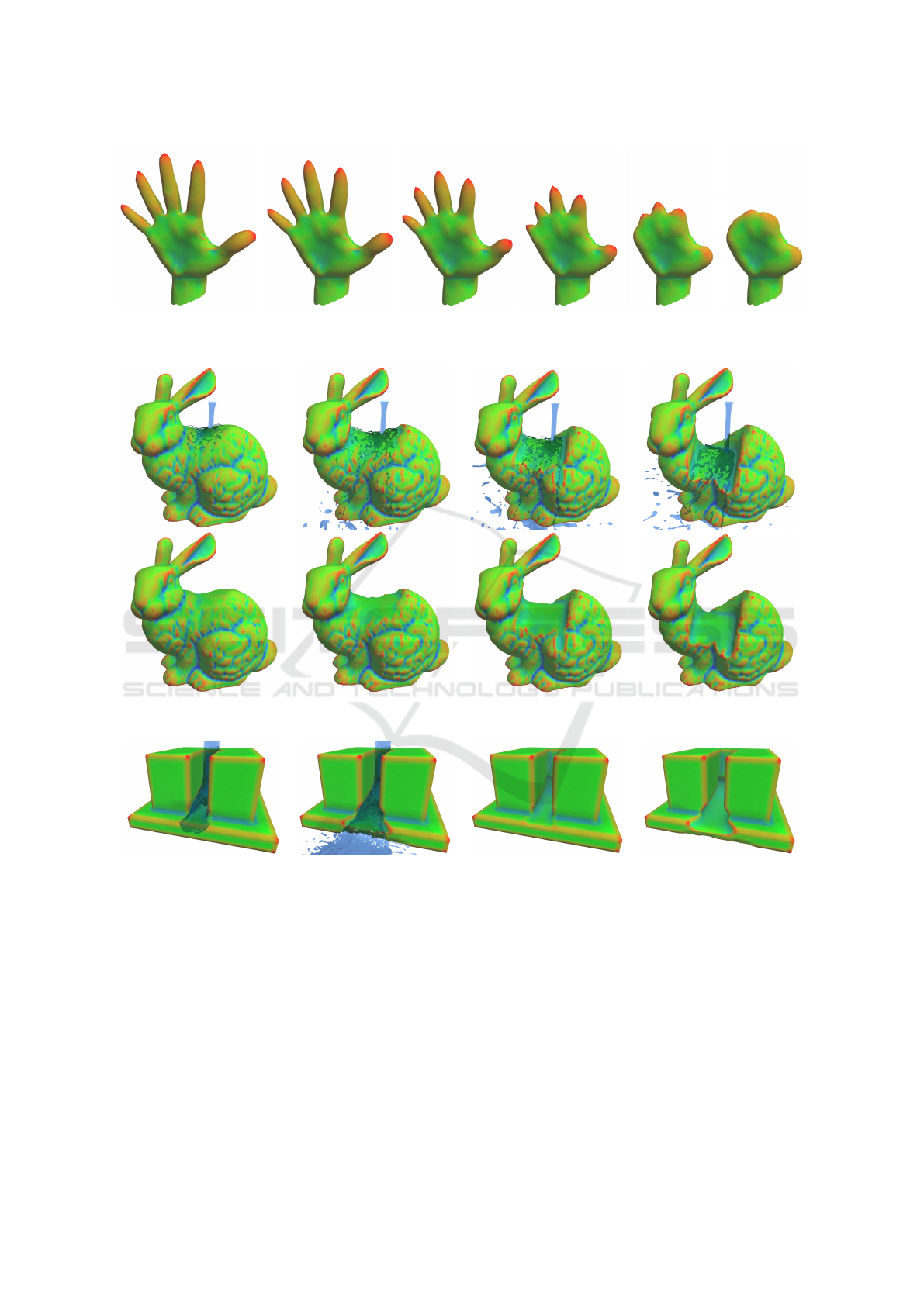
Figure 9: Weathering of a highly protruded model. Small faces are removed to prevent damaging the mesh. Left to right:

simulation after 20, 50, 100, 200, 300, and 400 iterations. Power modiﬁer n = 5; using curvature color coding as described in

Figure 2.

Figure 10: Hydraulic erosion simulation. Top: scene with simulated ﬂuid; bottom: isolated model. Left to right: model after

40, 200, 400, and 700 iterations. Using curvature color coding as described in Figure 2.

Figure 11: Pouring water through a narrow canyon. Left to right: scene with simulated ﬂuid after 100 and 150 iterations,

isolated model after 100 and 150 iterations. Using curvature color coding as described in Figure 2.

uniform mesh resampling followed by quadric edge

collapse decimation. Figure 14 captures both the orig-

inal triangulation and the data after preprocessing.

We simulated the process of creation of the under-

cuts in the river banks in the hydraulic erosion sce-

nario captured in Figure 1. We simulated the ero-

sion using the approach described in Section 3.4. The

scene was set up with the following parameters: the

power modiﬁer n = 1 and the region of inﬂuence

in f luence

of a particle was set to the average edge

length. The simulation results in the creation of un-

dermined river banks with distinct overhangs espe-

cially in the river bend regions, as demonstrated in

Figure 1 and Figure 15.

We used the same data to simulate the ﬂooding of

the area due to high amount of fast ﬂowing water in

the river. The scene was set up with the following pa-

rameters: the power modiﬁer n = 1 and the region of

inﬂuence d

in f luence

of a particle was set to triple the

average edge length. The increased region of inﬂu-

ence d

in f luence

results in smoothing the edges of the

river bed and creating more convincing results. Fig-

ures 16 and 17 show the original scene and the result

of the simulation after 100, 200 and 300 iterations.

A Uniﬁed Curvature-driven Approach for Weathering and Hydraulic Erosion Simulation on Triangular Meshes

129

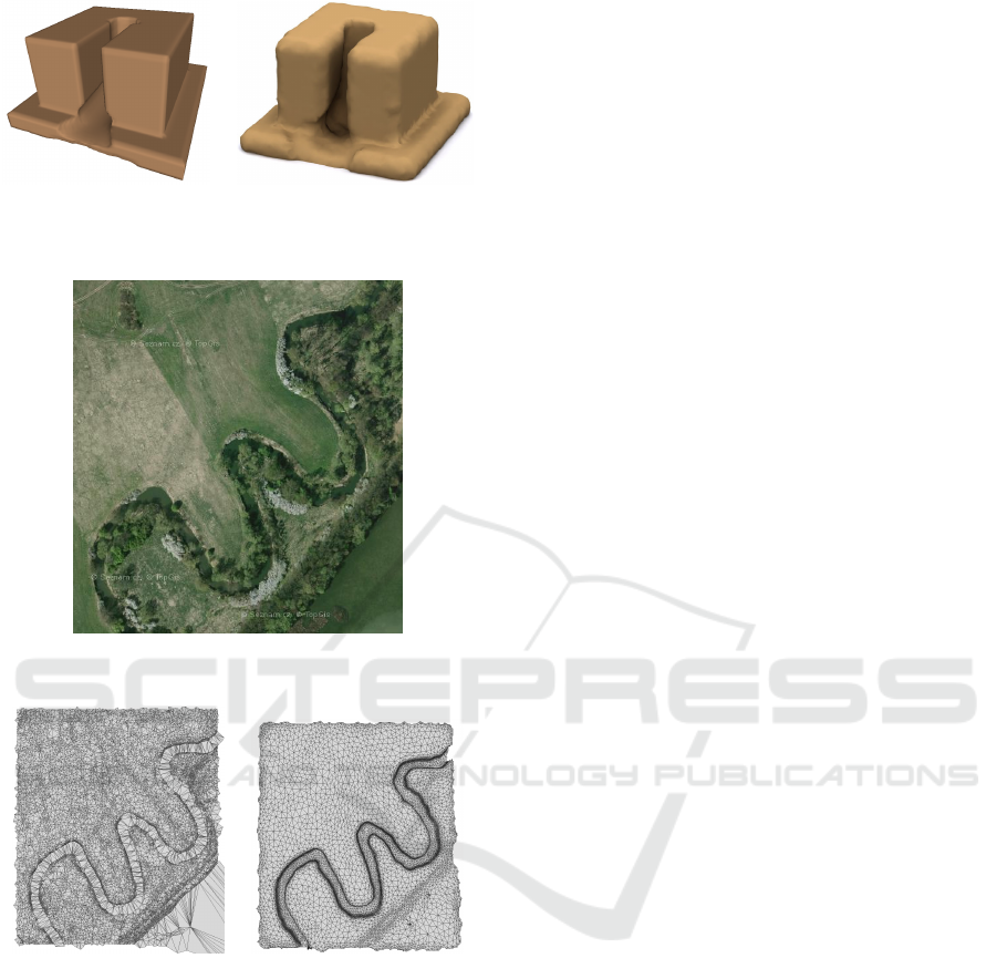
Figure 12: Pouring water through a narrow canyon.

Left: our approach; right: approach by Tychonievich and

Jones (Tychonievich and Jones, 2010).

Figure 13: River Odra in the Northern Moravia in the Czech

Republic. Source: www.Mapy.cz.

Figure 14: Triangulated lidar data (left) and the data after

preprocessing (right) of a river region captured in Figure 13.

Figure 18 captures the mean curvature of the original

scene and the ﬁnal scene after 300 iterations.

4.3 Execution Time

We have measured the execution time for the scenar-

ios presented in this Section on a computer equipped

by Intel i7-4770 3.4GHz, Intel HD Graphics 4600 and

16 GB RAM. We have measured the time required per

iteration of the method, as well as the execution time

of the most important substeps. The measured data

is shown in Tables 1 and 2 together with the num-

ber of vertices and faces of the corresponding scenes.

For hydraulic erosion scenarios captured in Table 2

we also record the average number of particles in the

scene. Even though we did not dedicate any special

effort to speed up the simulation, the simulation times

are very close to real-time frame rates. The real-time

simulation could be achieved by using more sophis-

ticated auxiliary structures or by implementing the

method on the GPU.

5 CONCLUSION

We have proposed a novel uniﬁed approach for the

two most prevalent erosion processes that can be ob-

served in nature, i. e., weathering and hydraulic ero-

sion. Our approach works directly with models repre-

sented as triangular meshes and simulates the erosion

by vertex displacement in the direction of the vertex

normal or the uniform discretization of the Laplace-

Beltrami operator, while the magnitude of the dis-

placement is calculated based on the local mean cur-

vature value.

The main advantage of our approach is that it of-

fers a uniﬁed way of simulating weathering and hy-

draulic erosion on triangular meshes, without the need

to employ other auxiliary intermediate data structures.

This allows us to use the simulation method on a wide

range of readily available triangular models. Trian-

gular meshes also permit to model complex scenes

with detailed features with varying density of vertices

based on the local complexity of the scene.

The use of triangular meshes and the simplicity of

the proposed method lead to very fast execution time

of the erosion simulation. We achieved almost inter-

active rates without deploying any special means to

speed up the algorithm. As future work, we would

like to achieve interactive simulation rates by per-

forming the erosion calculations on the GPU.

We have demonstrated our approach on both ar-

tiﬁcial and real data and showed that our method

results in the creation of visually plausible eroded

models despite the use of very simple erosion sim-

ulation function. To increase the plausibility of the

simulation, the erosion function could easily be re-

placed by more complex physically-based method.

Also, as future work, we would like to allow the

simulation of erosion of scenes composed of mul-

tiple materials by combining our approach with a

multi-material simulation approach, such as the ap-

proach by Skorkovsk

a and Kolingerov

a (Skorkovsk

and Kolingerov

a, 2016). Another obvious avenue for

this work is the handling of topological changes, such

as splitting the model in two due to heavy erosion.

GRAPP 2019 - 14th International Conference on Computer Graphics Theory and Applications

130

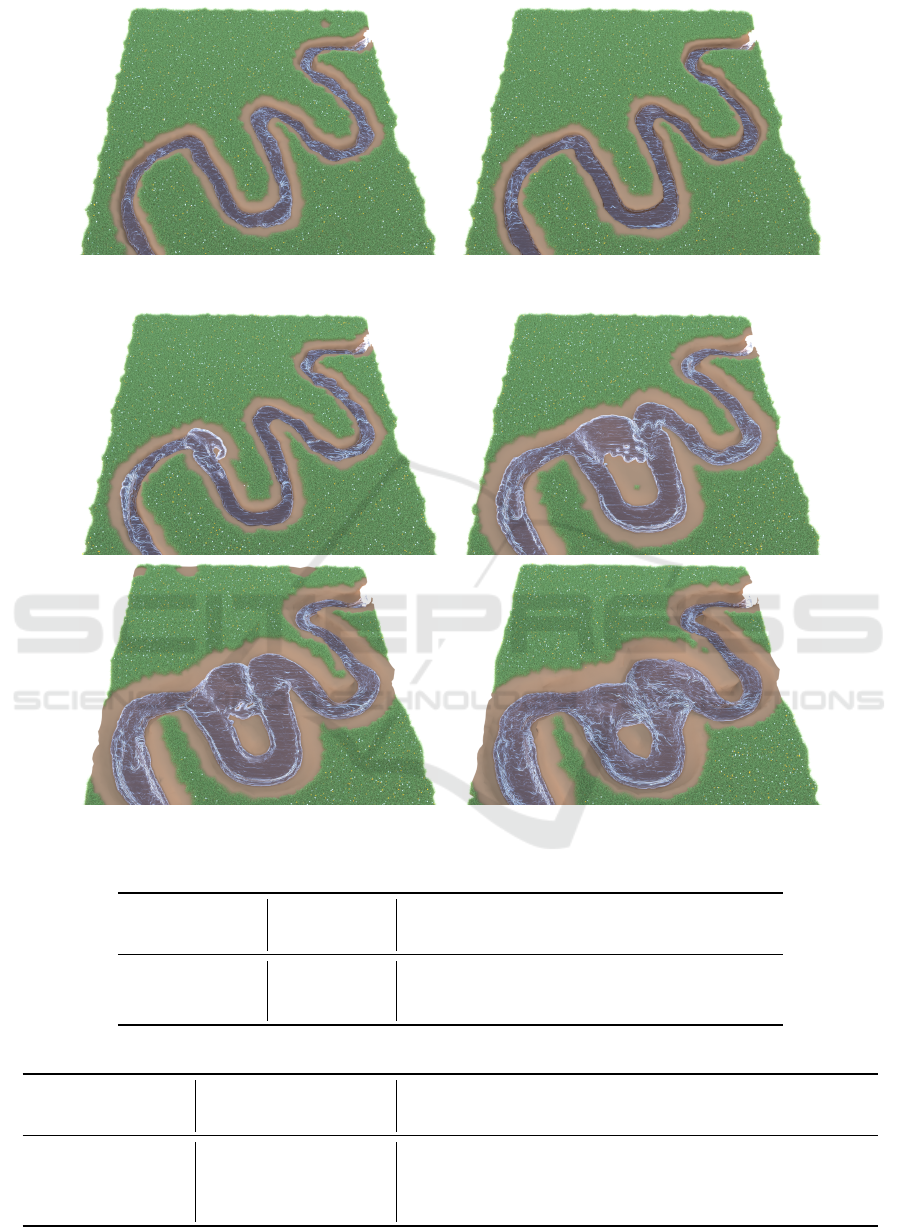
Figure 15: Running water creates undercuts on the river banks; top view. Original model (left) and the scene after 200

iterations (right) of hydraulic erosion simulation.

Figure 16: Fast water in the river erodes the river banks; top view. Top to bottom, left to right: original scene and the scene

after 100, 200, and 300 iterations.

Table 1: Size of the scene and execution time of steps of the algorithm (in ms) for the weathering simulations.

vertices faces iteration [ms]

curvature

calculation

[ms]

laplacian

calculation

[ms]

vertex

displacement

[ms]

Bunny (Figure 7) 34,835 69,666 182.705 144.571 16.167 0.354

Hand, n=1 (Figure 8) 2,518 5,000 27.464 9.907 1.234 0.028

Hand, n=10 (Figure 8) 2,518 5,000 27.556 9.855 1.218 0.034

Table 2: Size of the scene and execution time of steps of the algorithm (in ms) for the hydraulic erosion simulations.

vertices faces particles iteration [ms]

calculate

affected

vertices [ms]

curvature

calculation

[ms]

laplacian

calculation

[ms]

vertex

displacement

[ms]

Bunny (Figure 10) 34,835 69,666 17,673 291.520 34.601 150.006 15.528 1.713

Canyon (Figure 11) 17,130 34,256 67,561 309.441 116.228 63.749 6.069 0.834

River undercut (Figure 15) 7,806 14,782 72,569 271.863 117.651 28.374 3.171 0.528

River ﬂooding (Figure 16) 7,806 14,782 72,193 478.560 370.570 28.346 3.220 0.524

A Uniﬁed Curvature-driven Approach for Weathering and Hydraulic Erosion Simulation on Triangular Meshes

131

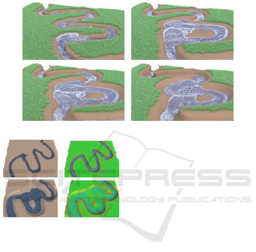
Figure 17: Fast water in the river erodes the river banks; front view. Top to bottom, left to right: original scene and the scene

after 100, 200, and 300 iterations.

Figure 18: Simple rendering (left) and mean curvature val-

ues (right) for the simulation in Figure 16 for original scene

(top) and the scene after 300 iterations (bottom). Using cur-

vature color coding as described in Figure 2.

ACKNOWLEDGEMENTS

This work has been supported by the project SGS-

2016-013 - Advanced Graphical and Computing Sys-

tems.

REFERENCES

Bene

s, B. (2007). Real-time erosion using shallow water

simulation. In VRIPHYS, pages 43–50. Eurographics

Association.

Bene

s, B. and Arriaga, X. (2005). Table mountains by vir-

tual erosion. In Poulin, P. and Galin, E., editors, Pro-

ceedings of the Eurographics Workshop on Natural

Phenomena, NPH 2005, pages 33–39. Eurographics

Association.

Bene

s, B. and Forsbach, R. (2002). Visual simulation of

hydraulic erosion. Journal of WSCG, pages 79–86.

Bene

s, B., T

ınsk

y, V., Horny

s, J., and Bhatia, S. K.

(2006). Hydraulic erosion. Computer Animation and

Virtual Worlds, 17(2):99–108.

Chiba, N., Muraoka, K., and Fujita, K. (1998). An erosion

model based on velocity ﬁelds for the visual simula-

tion of mountain scenery. The Journal of Visualization

and Computer Animation, 9(4):185–194.

Cignoni, P., Callieri, M., Corsini, M., Dellepiane, M.,

Ganovelli, F., and Ranzuglia, G. (2008). MeshLab:

an Open-Source Mesh Processing Tool. In Scarano,

V., Chiara, R. D., and Erra, U., editors, Eurographics

Italian Chapter Conference. The Eurographics Asso-

ciation.

Cordonnier, G., Braun, J., Cani, M.-P., Benes, B., Galin,

E., Peytavie, A., and Gu

erin, E. (2016). Large scale

terrain generation from tectonic uplift and ﬂuvial ero-

sion. In Proceedings of the 37th Annual Conference

of the European Association for Computer Graphics,

EG ’16, pages 165–175, Goslar Germany, Germany.

Eurographics Association.

Cordonnier, G., Galin, E., Gain, J., Benes, B., Gu

erin, E.,

Peytavie, A., and Cani, M.-P. (2017). Authoring land-

scapes by combining ecosystem and terrain erosion

simulation. ACM Trans. Graph., 36(4):134:1–134:12.

Crespin, B., B

ezin, R., Skapin, X., Terraz, O., and Meseure,

P. (2014). Generalized maps for erosion and sedimen-

tation simulation. Computers & Graphics, 45:1–16.

Dorsey, J., Edelman, A., Jensen, H. W., Legakis, J., and

Pedersen, H. K. (1999). Modeling and rendering

of weathered stone. In Proceedings of the 26th an-

nual conference on Computer graphics and inter-

active techniques, SIGGRAPH ’99, pages 225–234,

GRAPP 2019 - 14th International Conference on Computer Graphics Theory and Applications

132

New York, NY, USA. ACM Press/Addison-Wesley

Publishing Co.

Jones, M. D., Farley, M., Butler, J., and Beardall, M. (2010).

Directable weathering of concave rock using curva-

ture estimation. IEEE Transactions on Visualization

and Computer Graphics, 16:81–94.

Kri

stof, P., Bene

s, B., K

riv

anek, J., and

St’ava, O. (2009).

Hydraulic erosion using smoothed particle hydrody-

namics. In Computer Graphics Forum, volume 28,

pages 219–228. Wiley Online Library.

Levoy, M., Gerth, J., Curless, B., and Pull, K.

(2005). The stanford 3d scanning repository.

http://graphics.stanford.edu/data/3Dscanrep/.

Lienhardt, P. (1994). N-dimensional generalized combi-

natorial maps and cellular quasi-manifolds. Interna-

tional Journal of Computational Geometry & Appli-

cations, 4(03):275–324.

Mei, X., Decaudin, P., and Hu, B. (2007). Fast hydraulic

erosion simulation and visualization on gpu. In Pro-

ceedings of the 15th Paciﬁc Conference on Computer

Graphics and Applications, PG ’07, pages 47–56,

Washington, DC, USA. IEEE Computer Society.

Musgrave, F. K., Kolb, C. E., and Mace, R. S. (1989).

The synthesis and rendering of eroded fractal terrains.

SIGGRAPH Comput. Graph., 23(3):41–50.

NVIDIA (2014). Nvidia ﬂex. http://docs.nvidia.com/game

works/content/gameworkslibrary/physx/ﬂex/index.ht

ml. Online; Accessed: 01/04/2018.

Rusinkiewicz, S. (2004). Estimating curvatures and their

derivatives on triangle meshes. In Proceedings of

the 3D Data Processing, Visualization, and Trans-

mission, 2Nd International Symposium, 3DPVT ’04,

pages 486–493, Washington, DC, USA. IEEE Com-

puter Society.

Skorkovsk

a, V. and Kolingerov

a, I. (2016). Complex multi-

material approach for dynamic simulations. Comput-

ers & Graphics, 56:11 – 19.

Skorkovsk

a, V., Kolingerov

a, I., and Benes, B. (2015).

Hydraulic erosion modeling on a triangular mesh.

In R

ckov

a, K. and Inspektor, T., editors, Surface

Models for Geosciences, Lecture Notes in Geoinfor-

mation and Cartography, pages 237–247. Springer In-

ternational Publishing.

Tychonievich, L. A. and Jones, M. D. (2010). Delaunay

deformable mesh for the weathering and erosion of 3d

terrain. Vis. Comput., 26(12):1485–1495.

sa, L., Van

cek, P., Prantl, M., Skorkovsk

a, V., Mart

ınek,

P., and Kolingerov

a, I. (2016). Mesh statistics for ro-

bust curvature estimation. Computer Graphics Forum,

35(5):271–280.

Wojtan, C., Carlson, M., Mucha, P. J., and Turk, G. (2007).

Animating corrosion and erosion. In Proceedings of

the Eurographics Workshop on Natural Phenomena,

NPH 2007, pages 15–22. Eurographics Association.

A Uniﬁed Curvature-driven Approach for Weathering and Hydraulic Erosion Simulation on Triangular Meshes

133