Character Motion in Function Space

Innfarn Yoo

1,2

, Marek Fi

ser

, Kaimo Hu

and Bedrich Benes

Nvidia, Inc, U.S.A.

Purdue University, U.S.A.

Keywords:

Character Motion, Functional Principal Component Analysis, Orthonormal Basis Functions.

Abstract:

We address the problem of animated character motion representation and approximation by introducing a

novel form of motion expression in a function space. For a given set of motions, our method extracts a

set of orthonormal basis (ONB) functions. Each motion is then expressed as a vector in the ONB space or

approximated by a subset of the ONB functions. Inspired by the static PCA, our approach works with the

time-varying functions. The set of ONB functions is extracted from the input motions by using functional

principal component analysis (FPCA) and it has an optimal coverage of the input motions for the given input

set. We show the applications of the novel compact representation by providing a motion distance metric,

motion synthesis algorithm, and a motion level of detail. Not only we can represent a motion by using the

ONB; a new motion can be synthesized by optimizing connectivity of reconstructed motion functions, or by

interpolating motion vectors. The quality of the approximation of the reconstructed motion can be set by

deﬁning a number of ONB functions, and this property is also used to level of detail. Our representation

provides compression of the motion. Although we need to store the generated ONB that are unique for each

set of input motions, we show that the compression factor of our representation is higher than for commonly

used analytic function methods. Moreover, our approach also provides lower distortion rate.

1 INTRODUCTION

Articulated character motion editing, capturing,

searching, and synthesizing present important chal-

lenges in computer animation. On one hand, the

amount of produced motion data grows rapidly which

further exacerbates these challenges. On the other

hand, despite the enormous progress in this ﬁeld, the

existing methods still have limitations. Among them

the compact motion representation is one underlying

common problem. The motion data is usually stored

in its raw form as rotations and positions of the joints

(or velocities and accelerations) that is space consum-

ing and difﬁcult to process. One of the promising ap-

proaches is encoding the motion data by using ana-

lytic basis functions (e.g., Fourier, Legendre polyno-

mials, or spherical harmonics). These representations

compress the input data, but they may introduce un-

wanted artifacts such as oscillations, and may require

high number of basis functions to capture all details.

Moreover, synthesizing new motions from those rep-

resentations is difﬁcult.

A body of previous work addresses the problem of

motion synthesis. One class of methods uses motion

graphs for representing motion connectivity and syn-

thesizing new motions (Kovar et al., 2002a; Safonova

and Hodgins, 2007; Lee et al., 2010; Min and Chai,

2012). Functional analysis has been applied for en-

coding and searching motions (Unuma et al., 1995;

Ormoneit et al., 2005; Chao et al., 2012). Statisti-

cal approaches extract probabilities motion data with

the aim of low dimensional expression, predicting

smoothly connected motions (Ikemoto et al., 2009;

Lau et al., 2009; Wei et al., 2011; Levine et al., 2012),

and using physics-based representations to generate

new motions by simulation (Mordatch et al., 2010;

Wei et al., 2011). Although these methods are well-

suited for their particular area, they usually require

either a large amount of data to represent the motion,

or substantial effort for new motion synthesis.

Our work is motivated by advances in functional

data analysis and modeling in mathematics and statis-

tics (Ramsay and Silverman, 2006; Yao et al., 2005;

Coffey et al., 2011; Du et al., 2016). The key obser-

vation of our work is that for a given set of input mo-

tions, we can extract an optimal set of orthonormal

basis functions. While analytic basis functions have

been used for encoding motions, ours extracted ONB

functions are tailored for the given set of input mo-

tions and they are optimal in the sense that they pro-

110

Yoo, I., Fišer, M., Hu, K. and Benes, B.

Character Motion in Function Space.

DOI: 10.5220/0007456401100121

In Proceedings of the 14th International Joint Conference on Computer Vision, Imaging and Computer Graphics Theory and Applications (VISIGRAPP 2019), pages 110-121

ISBN: 978-989-758-354-4

Multi‐dimensional

FunctionSpace

Optimal

Function

Space

Optimal

Function

Space

…

SynthesisSynthesis

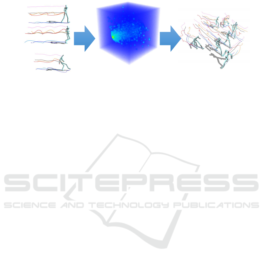
Figure 1: A set of raw motion data (left) is used to ﬁnd orthonormal basis functions by functional principal component analysis

(FPCA). Each input motion is encoded as a motion vector in the function space (center). While the novel representation

provides compression of the input data, the motion vectors synthesize new motions by interpolating their coordinates (right).

vide the best coverage for the range of the provided

input motions. Each input motion is then simply rep-

resented by its coordinates as a motion vector in the

ONB function inner-product space or approximated

by using a subset of ONB functions.

The input to our framework is a set of unlabeled

raw motion data of articulated characters, from mo-

tion capturing databases, hand-made animation, or re-

sults of physics-based simulation. In the ﬁrst step we

extract the ONB functions for the input set by using

functional principal component analysis (FPCA) and

represent each input motion as a motion vector in the

ONB space just by its coordinates. This compresses

the input data and converts it into a compact repre-

sentation. The vector representation of motions al-

lows for continuous (linear, or higher order) interpo-

lation in the inner-product space formed by the ONB

functions. We can synthesize a new motion sim-

ply by selecting two points in the ONB space, and

by interpolating between a successions of the closest

points between the two motions. However, for some

motions a simple interpolation might not be suitable

because they are dissimilar or far from each other.

For this case, we have adopted the connectivity op-

timization from Kovar et al. (2002a) to work for mo-

tion vectors in the ONB. In addition, this representa-

tion allows for the measure of distance between mo-

tions and it provides a compression of motion data.

Although we need to store the generated ONB that

are unique for input motions, the compression fac-

tor is higher than the commonly used analytic func-

tion methods. We claim the following contributions:

1) a novel representation of motions by extracting op-

timal orthonormal basis functions, 2) compact repre-

sentation of motions by encoding motions as motion

vectors into function space, 2) scalable motion recon-

struction so that can be used for level-of-detail (LOD),

and 4) motion synthesis via interpolation and partial

connectivity optimization in function domain.

2 PREVIOUS WORK

Function Analysis of Motion. The idea of repre-

senting motion in some other domain is rather old.

For example, the Fourier transform has been used fre-

quently in signal processing. Unuma et al. (1995) ap-

ply the Fourier transform to analyze, extract, and syn-

thesize motions by comparing existing motion data.

Ormoneit et al. (2005) detect cyclic behavior of hu-

man motions using function analysis and extract func-

tional principal components in the Fourier domain to

remove high frequency components. Similarly, Chao

et al. (2012) use spherical harmonic (SH) basis for

compressing and encoding motion trajectories. They

also retrieved similar motions by encoding and com-

paring user’s trajectory sketches. Coffey et al. (2011)

used PCA to analyze human motion data, but they did

not provide a way of synthesizing new ones. Du et

al. (2016) used scaled FPCA to adapt different types

of motion for character animation in gaming.

Our method does not use analytic orthonormal ba-

sis (ONB) functions, but we extract ad hoc ONB func-

tions from existing motion data. Our extracted ONB

functions are guaranteed to be optimal in a sense that

we can determine the error threshold and minimize

the error based on the number of ONB functions.

Motion Graphs. Kovar et al. (2002a) provide a

new distance metric of keyframes and introduce a

graph structure, called motion graphs, for motion

keyframes’ connectivity. Synthesizing a new motion

can be done by following a path in the graphs. Their

work extends in many directions. Lai et al (2005) use

motion graphs for small crowds by simulation and

constraints. Heck and Gleicher (2007) ﬁnd suitable

transitions of their parameterized motion space using

sampling methods. Reitsma and Pollard (2007) pro-

vide a task-based quality measure, such as different

types of motions, navigation ability, and embedding

additional data. Searching optimal interpolation path

Character Motion in Function Space

111

is researched in Safonova and Hodgins (2007). Beau-

doin et al. (2008) provide grouping of similar mo-

tions and construct a motif graph that allows search-

ing and constructing new motions. Zhao and Sa-

fonova (2009) improve the connectivity by construct-

ing well-connected motion graphs using interpolated

keyframes. Lee et al. (2010) show a novel method,

called motion ﬁelds, for interactively controlling lo-

comotion by introducing a new distance measure of

motions, which is combined with keyframe similarity

and velocity. Recently, Min and Chai (2012) com-

bined semantic information with motion graphs to

synthesize a new motion from simple sentences.

Our method represents motions as motion vectors

in an ONB function space and it allows for compact

motion representation and provides a distance met-

ric preservation. Also, an interpolation between any

two motions can be done by a simple vector interpola-

tion. We also generalize the optimization from motion

graphs for the ONB space.

Motion Clustering. Kovar et al. (2002a) generate

graph structures of motion data by calculating geo-

metric distances of motion keyframes. The motion

graphs were later extended in many ways, such as

by using different parametrization Kovar and Gle-

icher (2004); Heck and Gleicher (2007), they were

combined with clustering Beaudoin et al. (2008),

their connectivity was improved Zhao and Safonova

(2009), and optimal search was suggested Safonova

and Hodgins (2007), and their evaluations was in-

troduced in Reitsma and Pollard (2007). Barbi

c et

al. (2004) show three different approaches based on

PCA and Gaussian Mixture Model (GMM) for au-

tomatic segmentation of motion captured data. Our

method provides naturally deﬁned distance metric in

function space that allows for an easy calculation of

similarity of motions and clustering.

Motion Dimensionality Reduction. Mordatch et

al. (2010) developed a method that can perform user-

speciﬁed tasks by using Gaussian processes (GP) and

learning motions in reduced low-dimensional space.

Zhou and De la Torre (2012) extend the DTW method

by introducing Generalized Time Warping (GTW)

that overcomes DTW drawbacks for human motion

data. Ikemoto et al. (2009) exploit generalizations

of GP for motion data so that it allows users to edit

motion easily. Arikan suggested a motion compres-

sion method that is based on clustered principal com-

ponent analysis (CPCA) in Arikan (2006). Liu and

McMillan (2006) applied segmentation and PCA for

motion, and compressed the motion data. In addi-

tion, Tournier et al. (2009) provided a novel princi-

pal geodesic analysis (PGA), and achieved high com-

pression ratio. Although those PCA-based method

or dimensionality reduction methods studied in many

directions, there are several differences between our

method and the previous approaches. Our method

provides several additional properties such as motion

distance metric, level-of-detail, and fast reconstruc-

tion. Moreover, we interpret motions as a set of con-

tinuous functions so that it provides mathematically

well-deﬁned distance in function space. Also, our

method does not perform dimensionality reduction

and it allows for an easy motion synthesis by motion

vector interpolation or optimization.

3 OVERVIEW

Figure 2 shows an overview of our method that con-

sists of two parts: 1) function motion space construc-

tion and 1) motion synthesis. The input is a set of

input motions. During the ﬁrst step, we extract or-

thonormal basis functions (ONB) and represent (ap-

proximate if we do not use all ONB) each input mo-

tion as a motion vector that form a function motion

space. In the second phase, the motion vectors are

used to synthesize new motions.

The input character motion data stores positions

and rotations of joints and the data can originate from

motion capturing, physics-based animation, manual

creation, or similar. In the ﬁrst step we generate the

ONB by using functional principal component analy-

sis (FPCA) for all motions. Then, we obtain the co-

ordinates of each input motion in the ONB space. We

call the ONB encoded motions motion vectors, be-

cause they are represented only by their coordinates

in the corresponding ONB, and we call the set of en-

coded motions in the ONB the function motion space.

The resulting ONB and motion vectors are smaller

than the input data providing a compressed and com-

pact representation of the motions. Moreover, the

ONB representation allows for an easy motion syn-

thesis for each pair of vectors by simply interpolating

their coordinates. It is important to note that the ONB

form a space with a distance metric. We can therefore

measure the distance of two motions.

During the motion synthesis, the user deﬁnes the

start and the end of the motion by selecting two points

in the function motion space. The new motion can

be generated by interpolation, a process that is suit-

able for two closely positioned motions. If the points

are far from each other, we automatically traverse the

space and ﬁnd the shortest path between the closest

motion vectors, effectively combining the animations

together from the closest possible candidates. Using

a subset of the OBN or points that are too far can re-

sult in the combination of two motions that is not vi-

GRAPP 2019 - 14th International Conference on Computer Graphics Theory and Applications

112

FunctionMotionSpaceConstruction

Input

Motion

Database

FunctionalPrincipal

ComponentAnalysis

OrthonormalBasis

Functions

and

MotionVectors

Dynamic

TimeWarping

MotionSynthesis

Motion

Vectors

Selection

Motion

Interpolation

andOptimization

Synthesized

Motion

Time

Unwarping

Foot‐skating

Cleanup

Figure 2: An input set of motions is analyzed and an orthonormal basis is found by using functional principal component

analysis. The input motions are then encoded as a set of motion vectors in the ONB forming a function motion space. Novel

motion can be synthesized by interpolating through existing motion vectors or by optimization directly in the ONB.

sually plausible and introduce e.g., foot skating. In

this case we apply motion optimization from (Kovar

et al., 2002a) that has been modiﬁed and adapted to

work directly in the ONB.

4 ORTHONORMAL BASIS

FUNCTIONS AND MOTION

VECTORS EXTRACTION

The key idea of our approach is that an animated

character motion m(t) (see Section 5.3) can be rep-

resented as a vector with an optimal number of or-

thonormal basis function. Although, the idea of rep-

resenting motion data by using basis function has

been already used in computer graphics, previous ap-

proaches use given ﬁxed (analytic) basis functions

such as Fourier (e.g., Unuma et al. (1995)) or Spheri-

cal Harmonics (e.g., Chao et al. (2012)). Those func-

tions attempt to cover all possible motions by a set

of a priori given analytic basis functions. Not only

this representation is not optimal for a given input set,

but also the analytic basis functions may need a large

number of coefﬁcients to reduce oscillation of recon-

structed curves or to capture ﬁne details.

We use basis functions that are extracted from (a

group of) input motions. We use functional principal

component analysis (FPCA) to extract our basis that

covers the important motions in decreasing order. It

also provides the best coverage of the space by the

set of functions (see (Ramsay and Silverman, 2006;

Yao et al., 2005) for details of FPCA). In this section

we introduce the orthonormal function basis extrac-

tion and show how it is applied to motion encoding.

The function representation

f (t) is an approxima-

tion of a function f (t) and is expressed as

f (t) = µ(t) +

∑

i=0

(t), (1)

where µ(t) is the mean function represent-

ing the average of the analyzed functions,

B = {b

(t), b

(t), ...,b

(t)} is the ONB, and

,...,c

) are the coordinates of

f (t) in the

inner-product function space.

The error E(t) of the approximation is

E(t) = k f −

f k =



| f (s) −

f (s)|



1/2

. (2)

Having two ONB functions (motion vectors)

(t) = µ(t) +

∑

i=1

(t)

(t) = µ(t) +

∑

i=1

(t),

the distance D(

(t),

(t)) between them in the ONB

is calculated as the distance between two functions in

the given inner-product space (see 8):

(t),

(t)) =





(s) −

(s)





1/2



∑

i=1

−c

)



1/2



∑

i=1

−c

)



1/2

(3)

4.1 ONB Extraction using FPCA

The input to the ONB extraction is a set of K input

functions f

(t), k = 1,2,. ..,K. The f

(t) are time-

aligned components of the motion.We discretize func-

tions, f

) to Y

i j

with equally spaced time steps

i j

= f

) + ε

i j

, (4)

where ε

i j

is the measurement error per data point

(e.g., the error caused by motion capture).

The output of the ONB extraction is the set of

ONB functions b

(t) and the mean component

µ(t) =

∑

k=1

(t), ˆµ(t

i j

) =

∑

i=1

i j

. (5)

One of the important methods to extract orthonor-

mal basis in spatial domain is principal component

analysis (PCA) which maximizes space coverage for

a given number of basis function. Similarly, func-

tional principal component analysis (FPCA) (Ram-

say and Silverman, 2006) extracts ONB functions that

approximate the given set of functions. The FPCA

extract eigenfunctions that have maximal coverage

Character Motion in Function Space

113

of f

(t) and they are orthonormal to other eigenfunc-

tions in decreasing order of importance.

The FPCA uses the covariance function v(s,t)

v(s,t) =

∑

k=1

(s) f

(t).

To ﬁnd the basis b

(t), we ﬁnd Fredholm function

eigenequation that satisﬁes

v(s,t)b

(t)dt = ρb

(s) (6)

subject to hb

i = δ

i j

where δ

i j

is the Kronecker delta, ρ is an eigenvalue of

the principal component, the orthonormal basis b

(t)

is an eigenfunction, and the function inner-product

h f ,gi of two functions f (t) and g(t) is

h f

, f

i =

(s) f

(s)ds, (7)

where t

≤ t

< t

≤ t

. The raw covariances are cal-

culated as

i j

) = (Y

i j

− ˆµ(t

i j

))(Y

i j

− ˆµ(t

)),i 6= j

and the estimation v(s,t) is

˜v(s,t) =

∑

i=1

(s,t) =

∑

(s)

(t) (8)

where

λ is the estimated eigenvector, and

is the es-

timated eigenfunction. Since E(e

i j

) = 0 and the vari-

ance of error is

Var(e) = σ

the approximation of σ

can be estimated by

(

V (t) − ˜v(t,t))dt, (9)

where

V (t) is smoothed diagonal elements of ˜v

. The

eigenfunctions b

can be obtained by

−1

− ˆµ),

where

= ˜v +

Each eigenfunction b

(t) provides some coverage

of the input and the algorithm is executed until the the

average length of the residuals of the input is under

user-deﬁned percentage. This indirectly controls the

actual number of the ONB functions.

4.2 Coordinates in the ONB Function

Space

Having extracted the ONB b

(t) from f

(t), we can

represent each input function f

(t) in this space as

(t) with its coordinates (c

,...,c

) (see Eqn (1)).

The coordinates (c

,...,c

) are found by

= h f

i =

(s)b

(s)ds, (10)

where b

(t), b

(t), ...,b

(t) are the ONB functions.

The coordinates (c

,...,c

) are the coefﬁcients

that are the best approximation in the space formed

by the given ONB functions.

The ONB functions form a Hilbert space that has

vector space characteristics such as distance measure

and triangle inequality. A motion can be represented

as a linear combination of coefﬁcients (coordinates)

with ONB functions. Transition between two motions

is achieved by interpolating two motion vectors and

reconstructing the result back to the original motion

space. In addition, because of the nature of principal

component analysis, the order of orthonormal basis is

also the order of importance of the orthonormal axis.

5 CHARACTER MOTION

REPRESENTED AS

ORTHONORMAL BASIS

FUNCTIONS

We have shown how a function can be represented

by its coordinates in a function ONB space Eqn (1).

Moreover, we assumed there is a set of input func-

tions f

(t). From this input we extracted the ONB

(t) and each motion f

(t) is then represented (ap-

proximated) as

(t) by its coordinates c

. In this sec-

tion we show how a character motion can be repre-

sented by using ONB function representation.

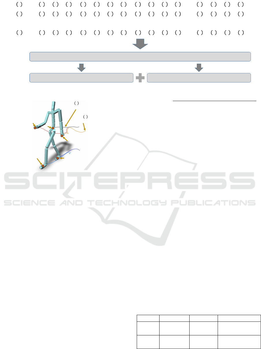
5.1 Skeleton and Motion

Representation

The input of our framework is an animated character

and we use notation from Lee and Shin (1999). The

articulated character is a skeleton hierarchy structure

(Figure 4) represented as a directed graph X = (J, E),

where J = { j

, j

,..., j

|J|

} are the joints (we use 31

joints in our experiments) and E = {e

,...,e

|E|

} is

a set of joint-index pairs. The root node of the hierar-

chy is denoted by j

and corresponds to the pelvis of

the character.

The articulated character motion is represented as

a set of translations of the root j

and the rotations of

each joint over time span t

,...,t

where m + 1 is

the number of the input motion poses. Although the

input is a set of discrete poses, we consider it a con-

tinuous function. The velocity of the root is denoted

GRAPP 2019 - 14th International Conference on Computer Graphics Theory and Applications

114





  



,



,



,



,



,



,



,



,



,



,



,⋯,



,



,



,





Re‐ordering&FPCA





  



,



,



,



,



,



,



,



,



,



,



,⋯,



,



,



,



 





  



,



,



,



,



,



,



,



,



,



,



,⋯,



,



,



,



 

⋮ ⋮⋮⋮⋮⋮⋮⋮ ⋮⋮⋮⋮ ⋮⋮⋮⋮

Eigenfunctions(ONBfunctions) MotionVectors

Figure 3: Per component ONB is extracted for different components of the input motion data.

𝑗

Root

𝑗

Right hand

𝑗

Left hand

𝑗

Left foot

𝑗

Right foot

𝑞

𝑡

Left hand joint rotation

𝑝 𝑡

root motion

Figure 4: Skeleton and joint curves labeling.

by ~v(t) and the rotation of each joint is q

(t). The

rotations of the joints are quaternions. The character

motion is a set

m(t) = {

v(t), q

(t), ...,q

(t)}, (11)

where ~v is the velocity vector of root position (with-

out initial yaw rotation) and q

(t) is the rotation of

joint j at the time t in the local coordinate system of

the skeleton. The world coordinates of the joint are

calculated by recursively traversing the skeleton from

the root j

and concatenating the corresponding rota-

tions and translations.

5.2 Dynamic Time Warping

Although two input motions are similar, they may

have different speed (time-scale). To solve the issue,

we ﬁrst calculate dynamic time warping (DTW)

input motions before extracting motion vectors and

ONB functions. We adopt the distance function be-

tween two keyframes by following (Lee et al., 2010)

d(m, m

) =

root

− v

root

( ˆu) −q

( ˆu)k

i=1

( ˆu) − p

( ˆu)k

i=1

k(q

)( ˆu)−(q

)( ˆu)k

(12)

where p is a positional unit quaternion, q is a unit

quaternion of a joint’s velocity, v is velocity vector

(see Eqn 13), β

is a weight of a joint, and p( ˆu) and

q( ˆu) mean rotation of arbitrary vector, ˆu. We use the

same weights for β

as in (Lee et al., 2010). In par-

ticular, we set the weight of the hip β

= 0.5 and

others β

,i = 1, ... ,k are set to the length of the cor-

responding bone lengths. The hip joint is the root

of skeleton hierarchy and it is important for overall

movement of the skeleton, so it has higher weight.

The velocity v of a pose can be calculated as

v = x

 x = (v

root

,...,q

)

= (x

root

− x

root

, p

−1

, p

−1

,..., p

−1

(13)

Based on the above keyframe distance, a DTW texture

is calculated for each pair of motions by accumulating

minimum distance as shown in Figure 6. The time

warping (time pairs from one to another) follows the

minimum distances in the given DTW texture. The

DTW improve the quality of FPCA and reduce the

number of basis functions (see Table 1).

Table 1: Error and Variance of FPCA result before and after

DTW (with precision of 0.9999). The DTW reduces the

error and the number of basis functions.

Avg Error Var. # of Basis Func

Before

DTW 0.003176 0.000079 10

After

DTW 0.002338 0.000088 6

Character Motion in Function Space

115

5.3 Motion as ONB

Let’s recall that the motion Eqn (11) has velocity of

the root ~v(t) and motion of each joint q

(t). The

components of ~v(t) = (~x(t),~y(t),~z(t)) and q

(t) =

(t), x

(t), y

(t), z

(t)) are used in the function anal-

ysis (Section 4) as 1D functions. Let’s denote f (t)

and g(t) as 1D functions corresponding to any pair

of the above-described components of motion. In the

following text we will not use the parameter t when-

ever it is clear from the context.

Figure 5: Closely matched motions that were calculated by

our approximated motion distance (Eqn 14): a) two soccer

kicking motions (0.022) and b) different walking motions

(0.007).

The ONB extraction needs a set of input functions.

We can construct the ONB for all motions by tak-

ing all components and running the algorithm from

Section 4. Let’s recall that the ONB generation is

executed until 0.999999 of variance is covered that

also deﬁnes the number of basis functions. Without

loss of generality we group motions as shown in Fig-

ure 3. For example, all components of root velocity~v,

and joints’ quaternions q

, are merged and then ONB

functions are extracted.

To calculate the distance between two motion

vectors, we account for the importance of joints in

motion distance calculation by associated weights

of each joint and we use the approach of Tang et

al. (2008) who deﬁned the joint weights. Let’s have

two motion vectors v

= {c

,...,c

} and v

,...,c

}. We use a modiﬁed distance equa-

tion that accounts for the above-mentioned weighting:

(t),

(t)) ≈



∑

i=1

− c

)



1/2

, (14)

where w

is the weights of joints. Fig 5 shows exam-

ples of closely matched two motion sequences.

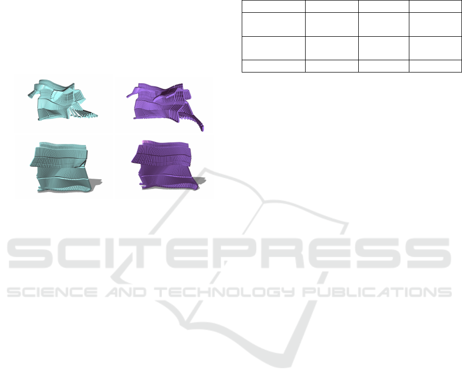
We experimented with three different ways of

combining functions for processing FPCA: a) per

component, b) per joint and per component, and c) all

functions together. As intuitively expected, collecting

Table 2: Average error, variance, and the required number

of basis functions for different conﬁguration. Comparison

of three different ways of FPCA processing: 1) per compo-

nent (velocities x, y, z and quaternion w, x, y, z), 2) per joint

and per component (velocity x, y, z, and per joint quaternion

w, x, y, z), and 3) all together.

Avg Error Variance # of Basis

Per

Component 0.002525 0.000093 114

Per Joint

Component 0.002140 0.000051 2032

All Together 0.002255 0.000084 23

functions per joint and per component provides best

quality (i.e., lowest error and lowest variance). How-

ever, the overall number of basis functions was too

high and it will lower the compression ratio. As a re-

sult, we combine all functions together and run FPCA

to extract ONB functions. It provides comparable er-

ror, but much smaller number of basis functions as

can be seen in Table 2.

We measured different sizes of ONBs in various

conﬁgurations. Our experimentations show that there

is no signiﬁcant difference if the motions are clustered

together in different ways, although a better insight

could be obtained by a careful evaluation.

6 MOTION SYNTHESIS USING

ONB

One advantage of the ONB representation is the in-

trinsic compression. Another advantage is the ease of

novel motion synthesis.

6.1 Motion Interpolation

Simple motion synthesis can be achieved by interpo-

lating two or more motion vectors, and then recon-

structing their spatial functions by using Eqn (1). This

corresponds exactly to a time step interpolation of the

original motions in the time domain, but it is achieved

in a very compact way simply as an interpolation of

the coordinates of motion vectors.

Let’s recall that the distance of motion vectors

is calculated by using Eqn (3). When n motions

are close enough, the interpolation and reconstruc-

tion create smooth motion transition between them.

In order to provide smooth interpolation of input mo-

tions, we calculate k nearest neighbors for each mo-

tion, and then provide the option to interpolate them.

If the points are close enough so that they belong to k

nearest neighbors, we apply B

ezier interpolation that

is suitable for short motion clip. In order to create

GRAPP 2019 - 14th International Conference on Computer Graphics Theory and Applications

116

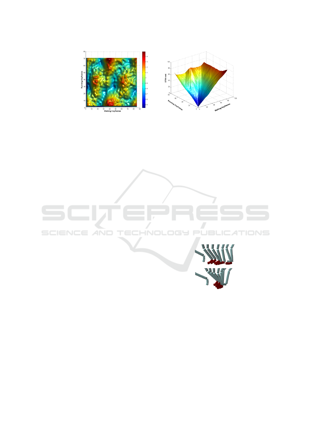
a) b)

Figure 6: A keyframe distance table is calculated by using Eqn 12. Then, minimum cost connectivity (time pairs) is calculated

by ﬁnding local minimum lines from the DTW texture.

longer sequences of motion, we need to connect the

motions by ﬁnding a partial connectivity of motion

clips.

6.2 Partial Similarity by Optimization

Some vectors can be too far to create a perceptually

good result. We compensate for this problem by op-

timization between the time sliding. We optimize

the objective function Eqn (15) that attempts to ﬁnd

scaling and sliding of time u and v from given inter-

val [t

] of two motions

argmin

u,v

∑

j=1



(us + v) −

(s)



ds =

argmin

u,v

∑

j=1



M(s) + A(s)



ds,

(15)

where N is the number of functions, M(s) = µ(us +

v) − µ(s), and A(s) =

∑

i=1

(us + v) − c

(s).

The resulting parameters u and v are the scaling and

sliding of time between two motions. This connectiv-

ity is similar to motion graphs (?). However, our ap-

proach is ﬁnding similar connectivity in inner-product

space, not keyframe distance in spatial domain.

6.3 Foot-skating Cleanup

The synthesized motions may contain foot-skating ar-

tifacts. We resolve this problem by detecting the foot-

plants and then smoothly adjusting the nearby root

and knee joint positions on their adjacent keyframes,

similar to (Ikemoto et al., 2006) and (Kovar et al.,

2002b).

The footplants are automatically detected from the

trained keyframes (Ikemoto et al., 2006). In the train-

ing process, the motion that contains the keyframe

with the farthest distance to the labeled keyframes

is selected for manual footplants marking. This it-

erative process terminates when the satisﬁed results

are achieved. In the detecting process, we calculate

the footplant values for each keyframe by averaging

the values of its k nearest neighbors in the trained

database.

Once the footplants are detected, we set the po-

sitions of the consecutive footplants as their average

values, and then smoothly relocate the root positions

of every keyframe in the sequence, such that their legs

are reachable to the positions. To avoid the pop-up

problems that may raise on the boundary of footplant

sequences, we linearly interpolate the root and foot

positions of the keyframes laying between the foot-

plants sequences. Additionally, the height of the root

for each keyframe is adjusted smoothly to make sure

its feet do not penetrate the ground. Finally, we ap-

ply the inverse kinematics on all the keyframes in the

synthesized motion.

Figure 7: The partial keyframe sequences before a) and after

foot-skating cleanup b). The adjacent keyframes containing

no footplants are also smoothly adjusted to avoid pop-up

problems.

7 IMPLEMENTATION AND

RESULTS

Our system is implemented in C++ and uses OpenGL

and GLSL to visualize results. All results were gen-

erated on an Intel



Xeon



E5-1650 CPU, running

at 3.20 GHz with 16 GB of memory, and rendered

Character Motion in Function Space

117

with an NVidia 970GTX GPU. All analysis and syn-

thesis computations were performed on a single CPU

thread. Initially, we used a FPCA library (PACE

package) that is implemented in Matlab. However,

it requires ﬁve hours to analyze 41 motions. To im-

prove the performance, we re-implement FPCA code

in C++ and by using CUDA. Our new implementation

provides signiﬁcantly faster performance than Matlab

PACE package, the achieved speedup is 10x for 210

curves and 225x for 6, 510 curves. Once the ONB

has been generated, the motion synthesis and decod-

ing are interactive.

7.1 FPCA CUDA Implementation

We use Eigen math library to represent matrices and

vectors, ALGLIB for spline smoothing, Armadillo

for fast singular value decomposition (SVD), and fast

Moore-Penrose pseudoinverse is implemented by fol-

lowing Courrieu’s method (Courrieu, 2008).

While the Matlab implementation is general, we

did not require all the functionality in our code. We

only consider special case which sampling points are

regular. In addition, we speed up FPCA processing

by applying CUDA for large-scale vector dot product

in Local Weighted Least Square (LWLS) estimation,

and removing cross-validation of residuals. Table 5

shows the comparisons of Matlab PACE package and

our implementation. The CUDA implementation will

be available on our web site.

Table 3: Average Error.

Test Case

Implementation 210 curves 6510 curves

PACE 0.00326511 0.00145804

Ours 0.00326484 0.00146001

Table 4: Max Error.

Test Case

Implementation 210 curves 6510 curves

PACE 0.06804195 0.20938692

Ours 0.06802791 0.20937758

Table 5: Processing Time (sec).

Test Case

Implementation 210 curves 6510 curves

PACE 24.2851400 784.976200

Ours 2.27931000 3.47349000

Comparison of FPCA implementations. Average error a),

maximum error b), and processing time c).

7.2 Evaluation

We compare our method against two other approaches

that use analytic basis functions: Fourier series and

Legendre polynomials. The advantage of the two ap-

proaches is that they do not need to store their an-

alytic basis functions because they are expressed as

equations. However, they generally need more coefﬁ-

cients to represent the function with the similar error

and the reconstruction artifacts are usually high fre-

quency oscillations that are unwanted in motion data.

Our method is less sensitive to these errors.

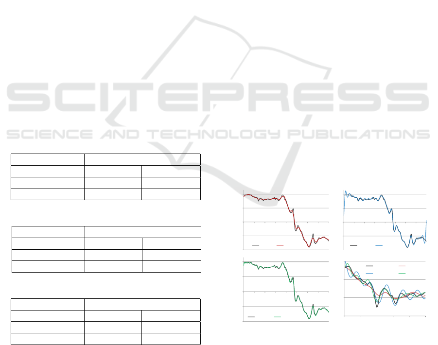
Reconstruction Comparison. We have used 41 mo-

tions and, in the ﬁrst step, we have generated the

ONB representation covering 0.999 of the variance

and measured the error of the approximation. In the

next step we encoded the same motion set by using

Fourier series and Legendre polynomials while en-

forcing the same error as for the ONB. The results

are displayed in Figure 8 where the Fourier series is

in green, Legendre polynomials blue, original motion

curve black, and our method in red. The approxima-

tion by using analytic functions introduces unwanted

oscillations as can be seen in the inset showing a de-

tailed span of 30-120 frames in Figure 8 d) and in the

accompanying video. This is due to the fact that the

high order basis functions have high frequencies that

would require more coefﬁcients to capture. In con-

trast, our basis functions adapt to the data and the re-

sulting reconstructed curve is smoother. At the same

time, while Fourier representation needed 476 basis

function and Legendre polynomials 293, our method

needed only 96 basis functions to approximate the

motion with the same error (see Table 6).

-0.2

-0.1

0.1

0.2

0 50 100 150 200 250 300 350

Original FPCA

-0.2

-0.1

0.1

0.2

0 50 100 150 200 250 300 350

Original Fourier (43)

-0.2

-0.1

0.1

0.2

0 50 100 150 200 250 300 350

Original Legendre (61)

0.14

0.16

0.18

0.2

30 50 70 90 110

Original FPCA

Fourier (43) Legendre (61)

Figure 8: Comparison of the original motion to our method

a), Fourier b), and Legendre c). Detail of 30-110 sec-

onds shows the analytic basis functions have higher oscil-

lations b) when encoded with the same error as our method.

Another advantage of our method is the control

over the error of the approximation. In our approach

GRAPP 2019 - 14th International Conference on Computer Graphics Theory and Applications

118

we do not need to specify the absolute error values.

We specify how much of the original information

should be preserved in the reconstructed curves and

run the corresponding ONB basis extraction. In all

experiments we set the error value to 0.1% (99.9%

quality).

Dimensions Comparison. We compared the space

needed for an accurate representation of all motion

curves per each component. We encoded all compo-

nent curves by using as few basis functions as possible

while making sure that 90th percentile error is below

a given error value. The comparison of the generated

number of basis vectors for our method, Fourier, and

Legendre is shown in Table 6. Overall our method

outperforms the other methods (96 : 476 with Fourier

and 96 : 293 to Legendre).

Table 6: Comparison of the required number of basis func-

tions.

90th percentile Number of basis functions

Comps. Our method Fourier Legendre

Total 96 476 293

Number of basis function for a given error.

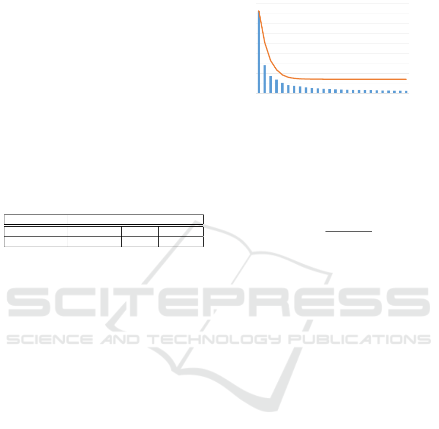
Compression. Our ONB function space representa-

tion of the character motion provides compression of

the input data. Although the basis functions are gen-

erated for each set of motions and they need to be

stored in order to reconstruct the motion, they outper-

formed Fourier and Legendre approximation in our

experiments as shown in Table 6.

We have encoded 321 different motions (2,605

short sequences, each of 0.8-1.2 seconds length at

120 Hz) that represented a skeleton with 31 joints.

The size of the raw input data is 227 MB. The com-

pression ratios depends on the number of basis func-

tions. In motion vectors, we do not store the vector

elements with the absolute values less than 1e-7. For

the ﬁrst 5 basis functions (mean function and the basis

functions), the compression ratios were 50× (see Fig-

ure 9), for Fourier 9×, and for Legendre polynomials

10×. The effect of the size of the ONB will further

diminish if more motions would be encoded and more

motion vectors would be present.

Our method cannot be directly compared to other

methods, such as (Arikan, 2006; Liu and McMillan,

2006; Tournier et al., 2009), since our method is not

used only for motion compressing, but it shares ONB

functions for further processing. In addition, the com-

pression ratio of our method can vary depending on

the number of used basis functions as shown in Fig 9.

Table 8 provides comparison of compression ra-

tio and distortion rate (%) based on the provided re-

sult from Liu and McMillan (2006) and Tournier et

0.002

0.004

0.006

0.008

0.01

0.012

0.014

0.016

100

150

200

250

300

350

400

450

1 3 5 7 9 11 13 15 17 19 21 23 25

AverageError

CompressionRatio

NumberofUsedONBFunctions

Error

CompressionRatio

Figure 9: The compression factor depends on the number

of basis functions. We removed motion vector elements

with the absolute values smaller than 1e-7 and calculated

the compression factors.

al. (2009). The same motion clips were used for

the comparison. The distortion rate is calculated by

Eqn (16) which was deﬁned by Karni and Gotsman

in (Karni and Gotsman, 2004).

d = 100

kA −

kA − E(A)k

, (16)

where A and

A are the 3m × n matrices that consist of

absolute markers’ position of original motion and the

decompressed motion respectively, m is the number

of markers, n is the number of keyframes, and E(A)

is the mean of marker positions with respect to time.

For reconstructing a frame, our method only requires

a few calculations by following Eqn (1) so that it can

reconstruct frames on the ﬂy.

8 CONCLUSION

We have introduced a novel compact representation

of motion for character animation. Our method is

inspired by analytic basis methods, such as Fourier

and Legendre polynomials, but instead of using an-

alytic representation the orthonormal basis (ONB) is

extracted automatically by using functional principal

analysis (FPCA) for each input set of motions. The

ONB is unique for each input set and because of the

FPCA the basis are ordered by their importance it

provides optimal coverage of the input space. Our

method not only provides better compression of the

raw input data than the analytic basis approximations,

it also allows for an easy motion synthesis. Each mo-

tion from the input set is represented as a motion vec-

tor and motion is performed by simply interpolating

motion vector coordinates and connecting partially

similar motions. We also provide optimization in the

ONB for more complex motions.

There are several limitations and avenues for fu-

ture work. One limitation is that the FPCA processes

Character Motion in Function Space

119

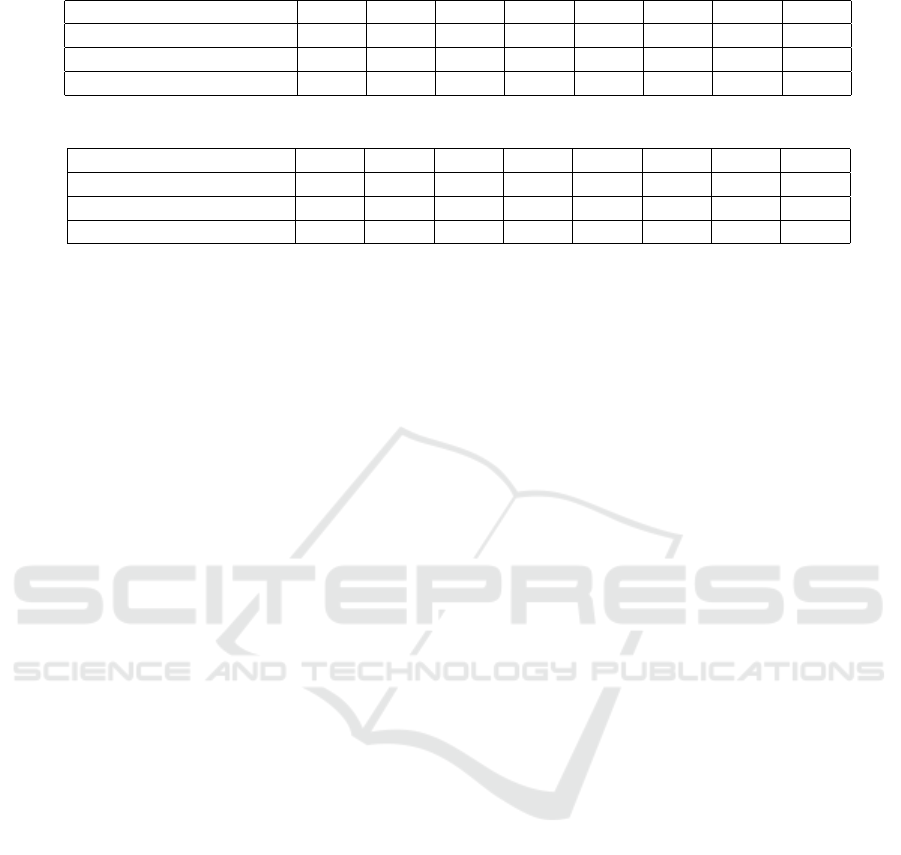
Table 7: Compression Ratio.

Method\Motion 09/06 13/29 15/04 17/08 17/10 85/12 86/02 86/08

Liu and McMillan (2006) N/A 1:55 N/A N/A N/A 1:18 1:53 1:56

Tournier et al. (2009) 1:18 N/A 1:69 1:182 1:61 1:97 N/A N/A

Ours (motion vector only) 1:19 1:33 1:63 1:34 1:33 1:34 1:34 1:29

Table 8: Distortion Rate (%).

Method\Motion 09/06 13/29 15/04 17/08 17/10 85/12 86/02 86/08

Liu and McMillan (2006) N/A 5.1 N/A N/A N/A 7.1 5.1 5.4

Tournier et al. (2009) 0.36 N/A 1.55 0.049 0.49 0.56 N/A N/A

Ours 1.11 0.30 0.21 0.39 0.23 0.34 0.38 0.40

The comparison between our method and other approaches. Note that we only used vector size for calculating compression

ratio, because our method the ONB functions are shared for all motions. In this table, lower than 1e-5 values are not saved,

and 6 basis functions were used.

only 1D functions. Theoretically, it would be possi-

ble to apply the FPCA directly to n-dimensional char-

acter animation and the per component optimizations

would not be necessary. Moreover, FPCA assumes

that the input functions are smooth, and also inter-

nally smooth the resulting ONB functions. As a side

effect, this could hide oscillations. Another limitation

is that the FPCA is always lossy due to numerical er-

rors in the computation.

ACKNOWLEDGEMENTS

The authors acknowledge the support of the OP

VVV MEYS funded project CZ.02.1.01/0.0/0.0/16

019/0000765 Research Center for Informatics.

REFERENCES

Arikan, O. (2006). Compression of motion capture

databases. ACM Trans. Graph., 25(3):890–897.

Barbi

c, J., Safonova, A., Pan, J.-Y., Faloutsos, C., Hodgins,

J. K., and Pollard, N. S. (2004). Segmenting motion

capture data into distinct behaviors. In Proceedings of

Graphics Interface 2004, pages 185–194.

Beaudoin, P., Coros, S., van de Panne, M., and Poulin, P.

(2008). Motion-motif graphs. In Proceedings SCA,

pages 117–126.

Chao, M.-W., Lin, C.-H., Assa, J., and Lee, T.-Y. (2012).

Human motion retrieval from hand-drawn sketch.

IEEE TVCG, 18(5):729–740.

Coffey, N., Harrison, A., Donoghue, O., and Hayes, K.

(2011). Common functional principal components

analysis: A new approach to analyzing human move-

ment data. Human Movement Science, 30(6):1144 –

1166.

Courrieu, P. (2008). Fast computation of moore-penrose

inverse matrices. CoRR, abs/0804.4809.

Du, H., Hosseini, S., Manns, M., Herrmann, E., and Fis-

cher, K. (2016). Scaled functional principal compo-

nent analysis for human motion synthesis. In Pro-

ceedings of the Intl. Conf. on Motion in Games, pages

139–144.

Heck, R. and Gleicher, M. (2007). Parametric motion

graphs. In Proceedings of the I3D.

Ikemoto, L., Arikan, O., and Forsyth, D. (2006). Knowing

when to put your foot down. In Proceedings of the

I3D, pages 49–53.

Ikemoto, L., Arikan, O., and Forsyth, D. (2009). Generaliz-

ing motion edits with gaussian processes. ACM Trans.

Graph., 28(1):1:1–1:12.

Karni, Z. and Gotsman, C. (2004). Compression of soft-

body animation sequences. Computers & Graphics,

28(1):25 – 34.

Kovar, L. and Gleicher, M. (2004). Automated extraction

and parameterization of motions in large data sets.

ACM Trans. Graph., 23(3):559–568.

Kovar, L., Gleicher, M., and Pighin, F. (2002a). Motion

graphs. ACM Trans. Graph., 21(3):473–482.

Kovar, L., Schreiner, J., and Gleicher, M. (2002b). Foot-

skate cleanup for motion capture editing. In Proceed-

ings of the SCA, pages 97–104.

Lai, Y.-C., Chenney, S., and Fan, S. (2005). Group motion

graphs. In Proceedings of the SCA, pages 281–290.

Lau, M., Bar-Joseph, Z., and Kuffner, J. (2009). Modeling

spatial and temporal variation in motion data. ACM

Trans. Graph., 28(5):171:1–171:10.

Lee, J. and Shin, S. Y. (1999). A hierarchical approach to

interactive motion editing for human-like ﬁgures. In

Proc. of the Annual Conf. on Comp. Graph. and Inter-

active Techniques, pages 39–48.

Lee, Y., Wampler, K., Bernstein, G., Popovi

c, J., and

Popovi

c, Z. (2010). Motion ﬁelds for interactive char-

acter locomotion. ACM Trans. Graph., 29(6):138:1–

138:8.

Levine, S., Wang, J. M., Haraux, A., Popovi

c, Z., and

Koltun, V. (2012). Continuous character control with

low-dimensional embeddings. ACM Trans. Graph.,

31(4):28:1–28:10.

Liu, G. and McMillan, L. (2006). Segment-based human

GRAPP 2019 - 14th International Conference on Computer Graphics Theory and Applications

120

motion compression. In Proceedings of the SCA,

pages 127–135.

Min, J. and Chai, J. (2012). Motion graphs++: A compact

generative model for semantic motion analysis and

synthesis. ACM Trans. Graph., 31(6):153:1–153:12.

Mordatch, I., de Lasa, M., and Hertzmann, A. (2010). Ro-

bust physics-based locomotion using low-dimensional

planning. ACM Trans. Graph., 29(4):71:1–71:8.

Ormoneit, D., Black, M. J., Hastie, T., and Kjellstrom,

H. (2005). Representing cyclic human motion us-

ing functional analysis. Image and Vision Computing,

23(14):1264 – 1276.

Ramsay, J. and Silverman, B. W. (2006). Functional data

analysis. Wiley Online Library.

Reitsma, P. S. A. and Pollard, N. S. (2007). Evaluating

motion graphs for character animation. ACM Trans.

Graph., 26(4).

Safonova, A. and Hodgins, J. K. (2007). Construction and

optimal search of interpolated motion graphs. ACM

Trans. Graph., 26(3).

Tang, J. K. T., Leung, H., Komura, T., and Shum, H. P. H.

(2008). Emulating human perception of motion simi-

larity. Computer Animation and Virtual Worlds, 19(3-

4):211–221.

Tournier, M., Wu, X., Courty, N., Arnaud, E., and

Revret, L. (2009). Motion compression using prin-

cipal geodesics analysis. Computer Graphics Forum,

28(2):355–364.

Unuma, M., Anjyo, K., and Takeuchi, R. (1995). Fourier

principles for emotion-based human ﬁgure animation.

In Proc. of the Annual Conf. on Comp. Graph. and

Interactive Techniques, pages 91–96.

Wei, X., Min, J., and Chai, J. (2011). Physically valid sta-

tistical models for human motion generation. ACM

Trans. Graph., 30(3):19:1–19:10.

Yao, F., Mueller, H.-G., and Wang, J.-L. (2005). Functional

linear regression analysis for longitudinal data. Ann.

Statist., 33(6):2873–2903.

Zhao, L. and Safonova, A. (2009). Achieving good connec-

tivity in motion graphs. Graphical Models, 71(4):139

– 152.

Zhou, F. and De la Torre, F. (2012). Generalized time warp-

ing for multi-modal alignment of human motion. In

IEEE Conference on CVPR, pages 1282–1289.

APPENDIX

Distance of Two Vectors in ONB Space

Let’s assume that two functions, f

(t) and f

(t),

are approximated by orthonormal basis functions,

(t), b

(t), ...,b

(t), so that the coefﬁcients are

,...,c

for

(t) and c

,...,c

for

(t).

The mean function of the two functions are µ(t),

so that the approximated functions,

(t) = µ(t) +

∑

i=1

(t) and

(t) = µ(t) +

∑

i=1

(t).

The squared distance between the two functions is

(t),

(t))



(s)−

(s)



ds =



∑

i=1

−c

(s)



Since b

(t), b

(t), ...,b

(t) are orthonor-

mal basis functions, any two basis func-

tions, b

(t) and b

(t) satisﬁes hb

i = δ

i j

where δ

i j

is kronecker delta function. Thus,



− c

(s) +··· + (c

− c

(s)



ds =

− c

)

(s)

ds + ··· +

− c

)

(s)

ds =

∑

i=1

− c

)

(s)

ds =

∑

i=1

− c

)

(s)

ds =

∑

i=1

− c

)

i =

∑

i=1

− c

)



The distance between two approximated functions is

just distance of their coefﬁcients.

Character Motion in Function Space

121