An MRF Optimisation Framework for Full 3D Helmholtz Stereopsis

Gianmarco Addari and Jean-Yves Guillemaut

Centre for Vision, Speech and Signal Processing, University of Surrey, Guildford, GU2 7XH, U.K.

Keywords:

3D Reconstruction, Helmholtz Stereopsis, Markov Random Fields.

Abstract:

Accurate 3D modelling of real world objects is essential in many applications such as digital ﬁlm production

and cultural heritage preservation. However, current modelling techniques rely on assumptions to constrain the

problem, effectively limiting the categories of scenes that can be reconstructed. A common assumption is that

the scene’s surface reﬂectance is Lambertian or known a priori. These constraints rarely hold true in practice

and result in inaccurate reconstructions. Helmholtz Stereopsis (HS) addresses this limitation by introducing a

reﬂectance agnostic modelling constraint, but prior work in this area has been predominantly limited to 2.5D

reconstruction, providing only a partial model of the scene. In contrast, this paper introduces the ﬁrst Markov

Random Field (MRF) optimisation framework for full 3D HS. First, an initial reconstruction is obtained

by performing 2.5D MRF optimisation with visibility constraints from multiple viewpoints and fusing the

different outputs. Then, a reﬁned 3D model is obtained through volumetric MRF optimisation using a tailored

Iterative Conditional Modes (ICM) algorithm. The proposed approach is evaluated with both synthetic and

real data. Results show that the proposed full 3D optimisation signiﬁcantly increases both geometric and

normal accuracy, being able to achieve sub-millimetre precision. Furthermore, the approach is shown to be

robust to occlusions and noise.

1 INTRODUCTION

Many industries such as ﬁlm, gaming and cultural

heritage require the ability to accurately digitise real

world objects. Despite signiﬁcant progress in 3D mo-

delling over the past decades, modelling scenes with

complex surface reﬂectance (e.g. glossy materials or

materials with spatially varying and anisotropic re-

ﬂectance properties) remains an open problem. Ex-

isting modelling techniques usually make simplifying

assumptions on the scene’s Bidirectional Reﬂectance

Distribution Function (BRDF) which fail to capture

the complexity of natural scenes. For instance, multi-

view stereo reconstruction techniques rely on the as-

sumption that the scene is Lambertian or sufﬁciently

textured to be able to use photo-consistency to in-

fer image correspondences across views. Photometric

Stereo (PS) can handle more complex types of sur-

face reﬂectance, but requires prior knowledge of the

BRDF, which is very difﬁcult to acquire in practice.

A solution to generalise 3D modelling to scenes

with complex reﬂectance has been proposed in the

form of Helmholtz Stereopsis (HS). The approach

utilises the principle of Helmholtz reciprocity to de-

rive a reconstruction methodology which is indepen-

dent of the scene’s surface reﬂectance. While very

promising results were demonstrated, previous for-

mulations of HS have been mostly limited to 2.5D

reconstruction (Zickler et al., 2002) (Roubtsova and

Guillemaut, 2018), thereby providing only a partial

scene reconstruction. Recently in (Delaunoy et al.,

2010), an approach was proposed to extend HS to the

3D domain, however, being based on gradient des-

cent, the approach is dependent on a good initiali-

sation to ensure convergence to the global optimum.

Overall, full 3D scene reconstruction using HS has re-

ceived limited consideration, with MRF formulations

limited to 2.5D scenarios.

This paper advances the state-of-the-art in model-

ling of scenes with arbitrary unknown surface reﬂec-

tance by proposing the ﬁrst Markov Random Field

(MRF) formulation of HS for full 3D scene recon-

struction. The paper makes two key contributions in

this area. First, it introduces a novel pipeline for full

3D modelling via fusion of 2.5D surface reconstructi-

ons obtained from multiple view-points through MRF

optimisation. Second, it proposes a volumetric MRF

formulation of HS that permits direct optimisation of

the complete 3D model and can be used to reﬁne the

previous estimate. Being based on an MRF formula-

tion, the approach is able to cope with coarse initiali-

sation and is robust to noise.

Addari, G. and Guillemaut, J.

An MRF Optimisation Framework for Full 3D Helmholtz Stereopsis.

DOI: 10.5220/0007407307250736

In Proceedings of the 14th International Joint Conference on Computer Vision, Imaging and Computer Graphics Theory and Applications (VISIGRAPP 2019), pages 725-736

ISBN: 978-989-758-354-4

725

2 RELATED WORK

The most common approaches to 3D reconstruction

are Shape from Silhouettes (SfS), multi-view stereo

and PS.

SfS was proposed in (Laurentini, 1994) and con-

sists in using 2D silhouette data to reconstruct a Vi-

sual Hull (VH) of the object. Despite having re-

cently been improved upon in recent works (Liang

and Wong, 2010) (Nasrin and Jabbar, 2015), SfS suf-

fers from being unable to reconstruct concavities.

Classic binocular and multi-view stereo approa-

ches (Szeliski et al., 2008) (Seitz et al., 2006) allow

for more complex geometric reconstructions than SfS,

but are limited by the scene BRDF, which needs to be

Lambertian. As this is often not the case, assuming

the wrong BRDF can lead to incorrect reconstructi-

ons. Some more recent multi-view techniques (Nis-

hino, 2009) (Oxholm and Nishino, 2016) (Lombardi

and Nishino, 2016) attempt to jointly estimate the ge-

ometry and reﬂectance models of the scene by cal-

culating iteratively the scene shape from the current

estimated reﬂectance and vice versa, which ultima-

tely constrains each calculation to the accuracy with

which the other parameter was estimated.

Finally, PS (Woodham, 1980) consists in compu-

ting the normals of a scene given a set of inputs with

stationary point of view but varying lighting. Despite

the possibility of reconstructing non-Lambertian sce-

nes, in PS the BRDF needs to be known a priori.

State-of-the-art work includes (Vogiatzis et al., 2006),

where a shiny, textureless object is reconstructed

using shadows and varying illumination, under the

simplifying assumption of a Lambertian reﬂectance

model. In (Chandraker et al., 2013) image derivatives

are used to reconstruct surfaces with unknown BRDF,

albeit being limited to isotropic BRDFs. In (Goldman

et al., 2010) a generic form of BRDF is used to com-

pute shapes, each point on the surface is considered to

be a mixture of previously calculated BRDFs, howe-

ver this is limited to a maximum of two materials per

point. In (Han and Shen, 2015), PS is computed for

isotropic and anisotropic reﬂectance models by consi-

dering the following characteristics of the BRDF: the

diffuse component, the concentration of specularities

and the resulting shadows. Despite achieving great

results, the set-up in this paper is extremely complex

and a large number of different light directions are

needed to perform the surface reconstruction.

The use of Helmholtz reciprocity (Von Helmholtz

and Southall, 1924) for 3D reconstruction was ﬁrst

proposed by Magda et al. in (Magda et al., 2001)

where the principle is used to recover the geometry

of scenes with arbitrary and anisotropic BRDF in a

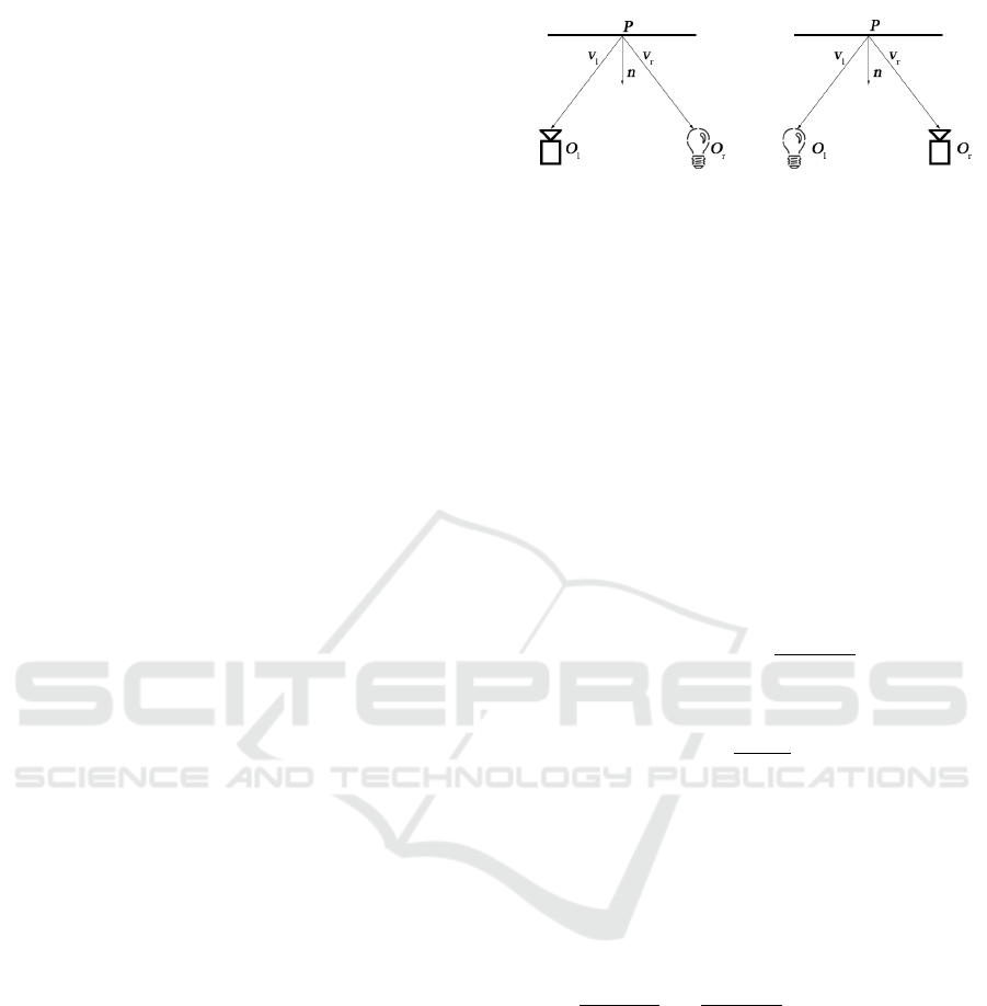
Figure 1: Camera/light pair positioning in HS.

simpliﬁed scenario. The proposed technique was then

further developed into HS in (Zickler et al., 2002)

by utilising it to perform normal estimation as well.

In the classical HS formulation maximum likelihood

is used to determine the depth of each point in the

scene, while the normals are estimated using Singu-

lar Value Decomposition (SVD). No integration is

performed over the surface, resulting in discontinui-

ties and a noisy reconstruction. To enforce Helmholtz

reciprocity, a set-up similar to the one shown in Fi-

gure 1 needs to be used. Let us consider a camera and

an isotropic, unit-strength point light source, respecti-

vely positioned at O

and O

. For a given surface point

P, the irradiance measured at its projection in the left

image (i

) can be expressed as:

= f

, v

) ·

n · v

− P|

(1)

where f

indicates the BRDF at point P with incident

light direction v

and viewing direction v

, n is the

surface normal at P and

−P|

accounts for the light

falloff. If the light and camera are interchanged, a

corresponding equation for the irradiance of the pro-

jection of P in the right image (i

) is obtained where

, v

) = f

, v

), due to the Helmholtz reciprocity

constraint. By performing a substitution, the reﬂec-

tance term can be removed and the following equa-

tion, independent from the surface BRDF, is obtai-

ned:



− P|

− i

− P|



· n = w · n = 0 (2)

Utilising multiple camera light pairs (at least

three) allows to obtain a matrix W where each row

is a w vector. By minimising the product W · n it is

possible to obtain an estimate of the normal at point

P. To do so the matrix is decomposed using SVD:

SV D(W) = UΣV

(3)

where Σ is a diagonal matrix and U and V are ortho-

gonal matrices. The last column of V gives an esti-

mate of the normal, while the non zero terms in the

diagonal matrix (σ

, σ

) can be used to compute a

quality measure of the normal.

In (Zickler et al., 2003) and (Tu and Mendonca,

2003) it is demonstrated that HS can be performed

VISAPP 2019 - 14th International Conference on Computer Vision Theory and Applications

726

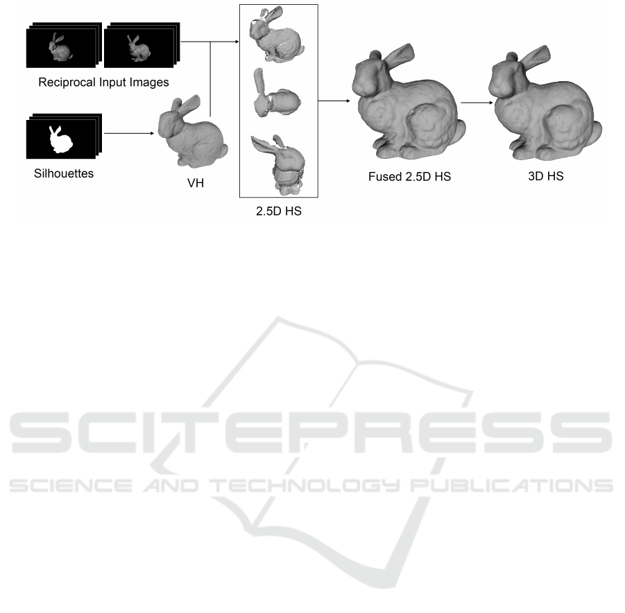
Figure 2: Pipeline overview.

with as low as a single pair of reciprocal images,

however the assumption of a C

continuous surface

is made, making it impossible to reconstruct surfa-

ces that present discontinuities. Further work include

(Guillemaut et al., 2004) where HS is applied to rough

and textured surfaces by integrating the image inten-

sities over small areas, (Janko et al., 2004) where it is

shown how performing radiometric scene calibration

allows for a vast improvement in the normal accuracy

calculated using HS, (Zickler, 2006) where geometric

and radiometric calibration are performed by exploi-

ting correspondences between the specular highlights

in the images and ﬁnally (Guillemaut et al., 2008)

where an alternative radiometric distance is proposed

to perform a maximum likelihood surface normal esti-

mation. All these methods are performed in 2.5D and

do not attempt to compute a globally optimal surface,

calculating instead an occupancy likelihood point by

point.

In (Roubtsova and Guillemaut, 2017) coloured

lights are used to reconstruct dynamic scenes using

only three cameras and a Bayesian formulation is pro-

posed to perform a globally optimal reconstruction

of the scene, while in (Roubtsova and Guillemaut,

2018) the maximum a posteriori formulation is app-

lied to classic HS by enforcing consistency between

the points depth and the estimated normals. This al-

lows to obtain less noisy results, however the scope

of these works is still restricted to 2.5D surfaces and

has not been applied to full 3D scenes. Furthermore,

occlusions are not handled by this method, affecting

its performance and severely restricting the scope of

scenes that can be reconstructed.

HS was ﬁrst applied in the 3D domain in (Wein-

mann et al., 2012), where it is used to complement

structured light consistency, which is unable to obtain

high frequency details on the reconstructed surface

and (Delaunoy et al., 2010), where a variational for-

mulation is presented to reconstruct a 3D mesh using

gradient descent optimisation. In Weinmann’s work

HS is only used as a reﬁnement step on areas of the

surface where ﬁne details are present and a very com-

plex set-up consisting of a light dome is used, which

makes this method extremely difﬁcult to deploy and

constrained to a speciﬁc set of scenes. In Delaunoy’s

work, instead, the set-up is simply a turntable, a pair

of ﬁxed lights and a ﬁxed camera, which makes it ea-

sier to reproduce. However, because the optimisation

employed is based on gradient descent, global opti-

mality is not guaranteed and the method could get

trapped in local minima if a proper initialisation is not

provided.

In contrast, the proposed method performs multi-

ple 2.5D reconstructions from different view-points,

which are then fused together to obtain a full 3D mo-

del of the scene. This is followed by an MRF opti-

misation on the 3D reconstruction, which, compared

to gradient descent, is less reliant on having a good

initialisation and beneﬁts from some optimality gua-

rantees depending on the choice of algorithm used to

optimise the energy function. During both steps self-

occlusions are taken into consideration by performing

an approximate visibility check.

3 PIPELINE OVERVIEW

In this section the pipeline used to perform the full

3D reconstruction is broken down, and each step is

detailed. As shown in Figure 2, the inputs to this met-

hod are calibrated Helmholtz reciprocal pairs of ima-

ges of the object and the silhouettes for each view.

The camera positions are arbitrary. The ﬁrst step con-

sists in deﬁning a voxel grid that contains the whole

object, and reconstructing its VH applying SfS to the

silhouettes.

An MRF Optimisation Framework for Full 3D Helmholtz Stereopsis

727

(a) (b)

Figure 3: Simpliﬁed representation of labelling in the 2.5D (a) and 3D (b) methods.

The VH is then used to initialise the next step,

where a set of separate views of the object are recon-

structed using a visibility aware Bayesian formulation

of HS. The approach extends the method from (Roub-

tsova and Guillemaut, 2018) with the use of additio-

nal information on visibility provided by the VH to

select a subset of cameras for each view and point in-

dependently. Selecting camera visibility correctly is

a critical step since the cameras are not all placed on

a plane as in other 2.5D Helmholtz methods, but can

instead be placed anywhere in the 3D space surroun-

ding the object, depending on how the dataset was

collected. In the proposed approach, reconstruction

is performed from the six viewing directions deﬁned

by the cardinal axes of the reference frame. These

deﬁne six orthographic virtual cameras and provide

sufﬁcient coverage to reconstruct the complete scene.

To remove redundancies and possible inconsisten-

cies among the partial surfaces, they are fused to-

gether using Poisson surface reconstruction. The re-

sulting surface is then used to initialise the ﬁnal step

of the reconstruction pipeline. In this ﬁnal step, the

problem is deﬁned as a volumetric MRF, where each

voxel corresponds to a node and the labelling deﬁnes

whether the node is outside, inside, or on the surface

of the reconstructed scene. A reﬁned 3D model is

obtained by MRF optimisation using a tailored Itera-

tive Conditional Modes (ICM) algorithm.

4 2.5D RECONSTRUCTION

FUSION

During this step multiple 2.5D depth maps of the ob-

ject are computed from different directions using HS

and optimised using MRF. Each problem is formu-

lated on an orthographic grid where each node corre-

sponds to an image point in the reference frame of

a virtual camera aligned with the chosen direction.

Each node can be assigned a label which indicates

the depth at which the surface is located at the cor-

responding pixel as shown in Figure 3a. The set of

labels is l

, ..., l

d−1

, where l

indicates the point in the

grid closest to the virtual camera and l

d−1

indicates

the farthest point in the grid. Each node is assigned a

label to minimise the following energy function:

E(l) = (1 − α)

∑

p∈I

(B(p,l

))+

∑

p,q∈N

(B(p,l

), B(q, l

)) (4)

where α is a balancing parameter between the data

and smoothness terms, I is the 2-dimensional grid de-

ﬁned by the virtual camera, D

(B(p,l

)) is the data

term of the function, which corresponds to the Helm-

holtz saliency measured at 3D point B(p, l

), obtained

by back-projecting image point P at the depth corre-

sponding to label l

. N

indicates the neighbour-

hood of a node, which consists of the four pixels di-

rectly adjacent in the image and S

(B(p,l

), B(q, l

))

is the smoothness term, and it corresponds to the nor-

mal consistency term calculated between 3D points

B(p, l

) and B(q, l

In this formulation the data term is computed

using the following equation:

(P) =

(

1, if |vis(P)| < min

vis

−µ×

(P)

, otherwise

(5)

where vis(P) indicates the set of reciprocal pairs of

cameras from which point P is visible, min

vis

is a vari-

able set to enforce the minimum number of reciprocal

pairs of cameras that make a normal estimate reliable,

µ is assigned the value 0.2 ln(2) to replicate the same

weight used in (Roubtsova and Guillemaut, 2018) and

and σ

are two values from the diagonal matrix

obtained performing SVD on matrix W as shown in

Equation 3.

VISAPP 2019 - 14th International Conference on Computer Vision Theory and Applications

728

Figure 4: Points on the surface (P) are approximated to the

closest point on the VH (P’) before occlusions are taken into

consideration for visibility.

An important contribution to enable application to

complex 3D scenes is the introduction of the visibility

term in the formulation. The ﬁrst criterion to deter-

mine visibility is to only consider the cameras whose

axis stands at an angle smaller than 80

◦

with respect

to the virtual camera axis. Then occlusions are com-

puted by approximating each point’s visibility based

on the visibility of its closest point on the surface of

the VH. If an intersection is found between the VH

and the segment connecting the camera center to the

approximated point, the camera and its reciprocal are

considered to be occluded and therefore are not used

as shown in Figure 4.

The smoothness function used here is the distance

based DNprior (Roubtsova and Guillemaut, 2018),

which enforces a smooth surface that is consistent

with the normals obtained through HS. This term is

calculated as follows:

(P, Q) =

(

(δ

P,Q

+ δ

Q,P

), if δ

P,Q

and δ

Q,P

< t

, otherwise

(6)

where t is the maximum threshold for δ

P,Q

. δ

P,Q

is the

distance between point P and the projection of Q, per-

pendicular to its estimated normal, on the grid pixel

where P lies as illustrated in Figure 5a, and it is cal-

culated as follows:

P,Q

PQ · n(Q)

n(Q) · C

(7)

where PQ is the vector connecting P and Q, n(Q) in-

dicates the estimated normal at point Q and C is the

virtual camera axis. Whenever δ

P,Q

or δ

Q,P

are grea-

ter than a threshold t dependent on the reconstruction

resolution, this term is truncated to t

in order to avoid

heavy penalties where a strong discontinuity is pre-

sent on the surface.

(a) (b)

Figure 5: Illustration of how S

(a) and S

(b) are com-

puted.

The energy function is then minimised using Tree

Reweighted Message Passing (TRW) (Kolmogorov,

2006) to obtain the depth maps from each viewing di-

rection. These are then fused together using Poisson

surface reconstruction (Kazhdan et al., 2006), and the

result is used to initialise the next step in the pipeline.

5 FULL 3D OPTIMISATION

In this step the reconstruction is further optimised in

full 3D. This is done by enforcing coherence between

neighbouring points in 3D, which is not guaranteed

when fusing partial depth maps obtained from diffe-

rent points of view. A 3D orthographic grid is created

that encompasses the whole object, and each voxel is

assigned a node in a multi-labelled MRF graph. The

labels are the following: {I, O, L

, ..., L

R−1

}, where I

and O indicate respectively whether the voxel is in-

side or outside the reconstructed surface, while the

remaining labels are assigned when the node is on

the surface. More speciﬁcally, the surface labels

, ..., L

R−1

} characterise the position of the surface

point in the local reference frame of each voxel. In

this paper, surface labels are deﬁned by regularly sam-

pling the interior of a voxel as shown in 3b, although

other sampling strategies could also be considered. In

this MRF formulation the following energy function

is minimised to optimise the surface:

E(L) = (1 − β)

∑

v∈V

(v, L

∑

v,w∈N

(v, L

, w, L

) (8)

where β is a weight to balance the effects of the data

and smoothness terms, V is the 3D grid and N

the neighbourhood composed by the six voxels di-

rectly adjacent to the current one. M(v, L

) indicates

the position of the surface point at node v when assig-

ned label L

. The data term is computed differently

depending on whether the point is inside, outside or

An MRF Optimisation Framework for Full 3D Helmholtz Stereopsis

729

on the surface:

(v, L

) =

(

0, L

∈ {I, O}

−µ×

(M(v,L

))

(M(v,L

))

, otherwise

(9)

Similarly to the data term, the way the smoothness

term is computed depends on the label combination of

the two nodes:

(v, L

, w, L

) =











Γ(M(v, L

), M(w, L

)), L

, L

∈ {L

, . . . , L

R−1

}

∞, L

, L

∈ {I, O}, L

6= L

0, otherwise

(10)

where

Γ(V, W) =

(γ

V,W

+ γ

W,V

) (11)

indicates the normal consistency in the 3D optimisa-

tion between points V and W. γ

V,W

is calculated as

follows:

V,W

= |VW · n(W)| (12)

where VW is the vector connecting points V and W,

while n(W) indicates the unit normal estimated via

HS at point W. This term consists of the distance be-

tween W and the plane perpendicular to n(V) inter-

secting point V. In Figure 5b an illustration of how

this term is calculated is shown. The ∞ term is here

used to constrain inside and outside voxels to be se-

parated by surface voxels, thus avoiding an empty so-

lution where all nodes are either labelled to be inside

or outside. The normal consistency term does not re-

quire truncation in the 3D domain.

Once the graph is initialised, the optimisation is

performed using a tailored version of ICM (Besag,

1986). ICM is an exhaustive search algorithm that ite-

rates through an MRF graph and changes one variable

at a time by trying to optimise its local neighbourhood

cost. In its classic formulation, ICM would not work

in this scenario because of the constraint on the sur-

face. Namely, changing the label of a surface node to

be either outside or inside would result in a hole on

the surface, which is currently prevented by having

an inﬁnite weight when outside and inside voxels are

neighbours. However, by changing two neighbouring

variables at a time, and considering all neighbouring

nodes to at least one of the two variables, the surface

can be shifted close to its optimal solution through

multiple iterations. Only tuples where one node is on

the current surface of the reconstruction are conside-

red, and for each tuple and their neighbours, all possi-

ble conﬁgurations are considered, selecting the solu-

tion with the lowest energy. Since the problem is ini-

tialised close to the actual surface, this step typically

converges after a small number of iterations. Finally,

the nodes labelled to be on the surface are extracted

together with their Helmholtz estimated normals and

are integrated using Poisson surface reconstruction to

obtain a mesh representation.

6 EVALUATION

In this section a brief description of the datasets used

to perform the evaluation is given, followed by an

analysis on the results obtained. The methods used

will hereby be denoted as follows: ‘VH’ for the recon-

struction obtained using SfS, ‘2.5D HS’ for the 2.5D

reconstructions obtained using the approach descri-

bed in Section 4, ‘Fused 2.5D HS’ for the fusion of

the 2.5D surfaces obtained using ‘2.5D HS’ and ‘3D

HS’ for the proposed method that performs MRF op-

timisation on the full 3D surface. Where available,

the ground truth is labelled ‘GT’.

6.1 Dataset

To test the methodology, both synthetic and real sce-

nes were used. It is important to note that, when gene-

rating synthetic scenes, commonly used rendering pi-

pelines often break Helmholtz reciprocity, providing

images that are not physically plausible. To address

this, synthetic images were rendered using the mo-

diﬁed Phong reﬂectance model (Lewis, 1994), which

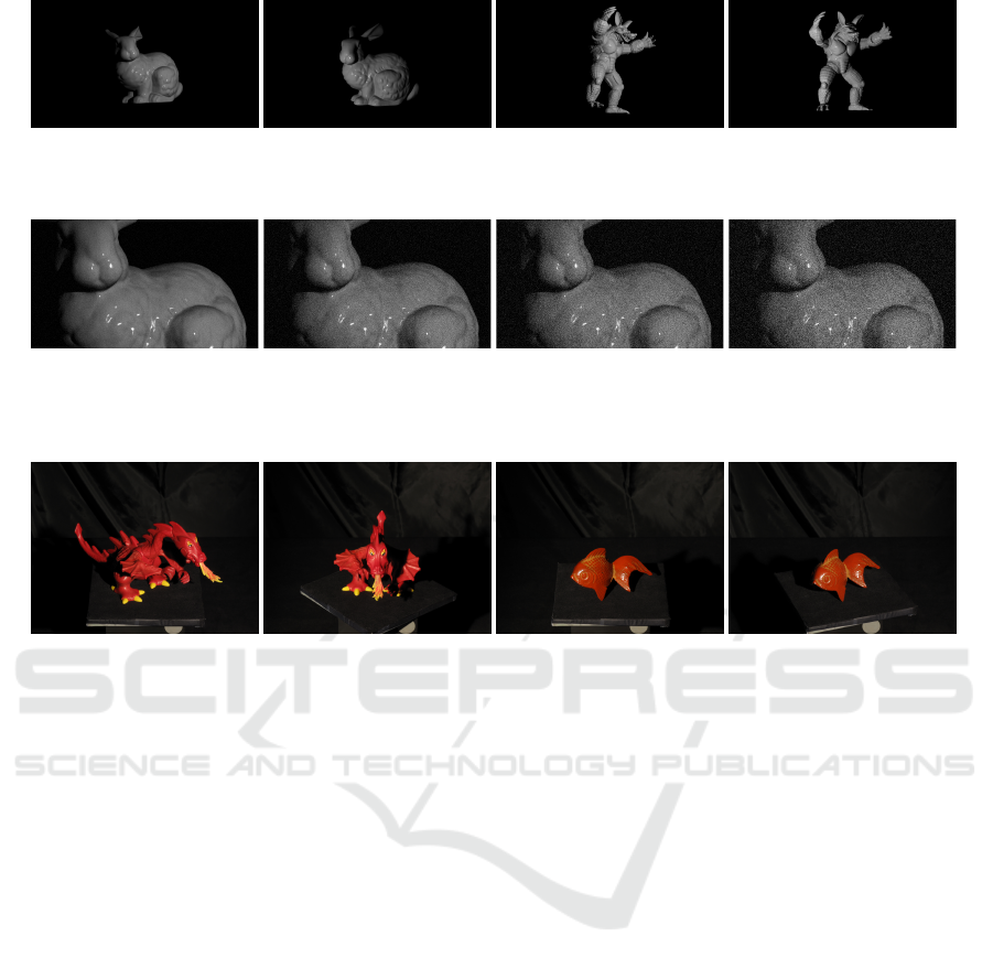
combines a diffuse and a specular part. In Figure 6

two reciprocal pairs of images are shown for the Stan-

ford Bunny (Turk and Levoy, 1994) and Armadillo

scenes (Krishnamurthy and Levoy, 1996). These sce-

nes were chosen because they both present elongated

thin structures, namely the ears of the bunny and the

limbs and claws of the armadillo; strong specularities

with no textures; and numerous self occlusions. The

synthetic scenes were also distorted to measure the ro-

bustness of the methodology against noisy input data.

In Figure 7 a close up of the distorted images used for

the experiments are shown.

Each scene is composed of 40 reciprocal pairs of

images captured from a set of viewpoints obtained

sampling a sphere around the object. The images are

rendered at a resolution of 1920 × 1080. Using synt-

hetic scenes allows for a quantitative evaluation of

the methodology, by comparing the results obtained

against the ground truth data.

The real dataset from (Delaunoy et al., 2010) is

composed of two scenes called Dragon and Fish. Two

reciprocal pairs of images are shown in Figure 8.

These two datasets are challenging due to the strong

specularities present on the surface of ‘Fish’ and the

VISAPP 2019 - 14th International Conference on Computer Vision Theory and Applications

730

(a) (b)

Figure 6: Two reciprocal pairs from the synthetic dataset: ‘Bunny’ (a) and ‘Armadillo’ (b).

(a) (b) (c) (d)

Figure 7: Images with added input noise (white noise with normalised standard deviation 0.001 (a), 0.005 (b), 0.010 (c), 0.020

(d)).

(a) (b)

Figure 8: Two reciprocal pairs from the real dataset: ‘Dragon’ (a) and ‘Fish’ (b).

numerous self occlusions in ‘Dragon’. It must be no-

ted that no ground truth data or laser scan is available

for these datasets, and thus only a qualitative evalua-

tion could be performed. The resolution of the ima-

ges from these scenes is 1104 × 828 and they are all

from a single ring of cameras positioned on top of the

objects, which means that one side of the object is al-

ways completely occluded. This is relevant to show

how the reconstruction method used is able to deal

with a lack of data.

6.2 Results

6.2.1 Synthetic Scenes

In this section a comparison between ‘VH’, ’Fused

2.5D HS’ and ‘3D HS’ is performed on the synthetic

scenes to quantitatively assess the performance of the

proposed approach compared to the state-of-the-art

2.5D technique. It was decided to compare the pro-

posed methodology directly against ‘Fused 2.5D HS’

because ‘2.5D HS’ produces only partial reconstructi-

ons of the object using a limited number of views. The

parameters used to measure performance are accuracy

at 90% and completeness calculated at different thres-

holds depending on the scene examined. The thres-

holds are chosen depending on the VH accuracy, to

measure whether there are holes in the reconstructed

mesh or areas where the accuracy is signiﬁcantly de-

graded.

In Figure 9 the results obtained from each met-

hod are shown. The results reported in this paper

were obtained using the following parameters: {α =

0.3, β = 0.4, t = 3 × r} where r is the edge length

of a pixel in the reference frame. Starting from the

left the initial VH is shown, followed by some of

the results obtained using ‘2.5D HS’. Being a view-

dependent approach, this method is limited to recon-

structing only parts of the surface which are directly

visible from the virtual camera. This produces ho-

les whenever a partial occlusion is found, as observed

in the lateral reconstructions of the arms in the ‘Ar-

madillo’ scene. Furthermore, surfaces which are hea-

vily slanted with respect to the viewing direction will

result in gaps in the reconstructed model, as shown

in the ‘2.5D HS’ upper right result of the ‘Bunny’

scene. ‘Fused 2.5D HS’ allows to tackle these pro-

blems by fusing together different views, but is prone

to artefacts where non matching surfaces are united.

This is mitigated by the use of Poisson surface re-

construction, which tends to smooth these artefacts,

however some of them are still visible in the results.

An MRF Optimisation Framework for Full 3D Helmholtz Stereopsis

731

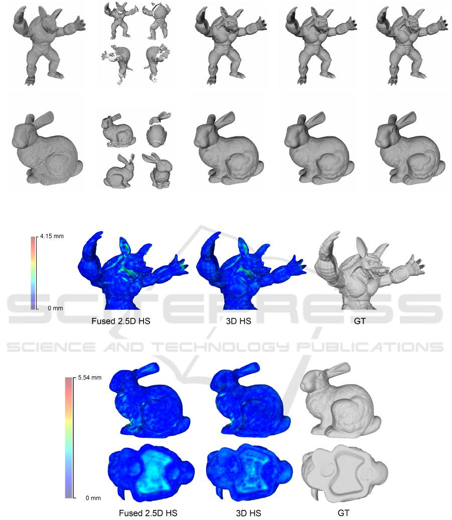
VH 2.5D HS Fused 2.5D HS 3D HS GT

Figure 9: Results from the ‘Armadillo’ and ‘Bunny’ scenes.

Figure 10: Heatmap showing the accuracy obtained by ‘Fused 2.5D HS’ and ‘3D HS’ when reconstructing the ‘Armadillo’

scene.

Figure 11: Heatmap showing the accuracy obtained by ‘Fused 2.5D HS’ and ‘3D HS’ when reconstructing the ‘Bunny’ scene.

Finally, ‘3D HS’ is used to perform a full 3D optimi-

sation on top of the previous steps, correcting these

artefacts and improving the overall accuracy of the

mesh. The results from all the different techniques

can be qualitatively compared with the ground truth

in the same ﬁgure.

In Figure 10 and 11 heatmaps are used to highlight

some details of the results where the reconstruction

accuracy is improved by ‘3D HS’ with respect to ‘Fu-

sed 2.5D HS’. In particular, concavities with a strong

error are improved upon by using ‘3D HS’, some no-

table parts where this can be observed are the ears of

the animals in both scenes and the concavity at the

base of the ‘Bunny’ scene.

VISAPP 2019 - 14th International Conference on Computer Vision Theory and Applications

732

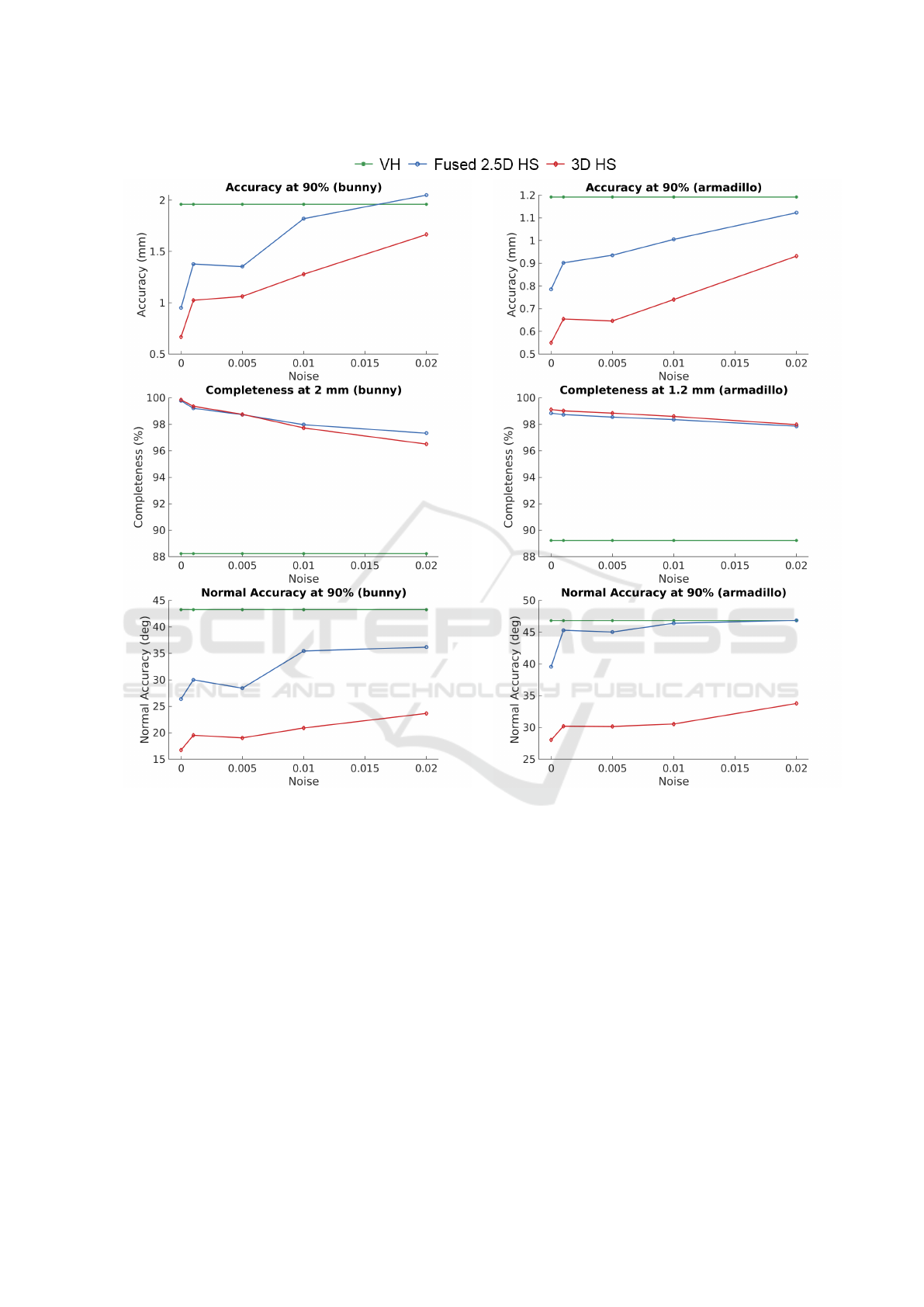
Figure 12: Graphs representing the results on the ‘Bunny’ and ‘Armadillo’ scene, including accuracy, completeness and

normal accuracy.

Finally, in Figure 12 the performance of these

methods is objectively measured at different levels

of input noise in terms of accuracy at 90%, normal

accuracy at 90% and completeness. As shown in the

graphs, ‘3D HS’ achieves sub-millimetre accuracy in

both scenes, exceeding ‘Fused 2.5D HS’ performance

by a signiﬁcant amount. In particular, in the ‘Arma-

dillo’ scene, which is characterised by a high number

of self-occlusions, ‘3D HS’ obtains exceptional re-

sults when compared with ‘Fused 2.5D HS’. In terms

of completeness, both techniques are able to recon-

struct the scene properly, without any holes or parts

with signiﬁcant loss of accuracy. In terms of normal

accuracy, ‘3D HS’ outperforms ‘Fused 2.5D HS’, and

in particular in the ‘Armadillo’ scene, which presents

high frequency details where it is hard to obtain very

precise normals.

The geometric and normal accuracy performance

degrades linearly with the introduction of noise, still

maintaining good results when the input images are

distorted with strong Gaussian noise with a normali-

sed standard deviation of 0.02. This indicates that the

approach is robust to noise. In particular, the normal

accuracy does not vary signiﬁcantly, showing how HS

normal estimation is robust to noise.

6.2.2 Real Scenes

Figure 13 shows the results obtained in the case of the

real scenes. These scene were reconstructed using a

very weak initialisation, as can be seen from the ‘VH’

An MRF Optimisation Framework for Full 3D Helmholtz Stereopsis

733

VH Fused 2.5D HS 3D HS Input Image

Figure 13: Results from the ‘Fish’ and ‘Dragon’ scenes.

results, due to a lack of precise silhouettes. Starting

from this coarse initialisation, the scene is ﬁrst recon-

structed from multiple view points in ‘2.5D HS’, and

then the fused depth maps are optimised using ‘3D

HS’, leading to accurate models that are able to cap-

ture ﬁne structural details including thin structures.

As can be observed from the results, the mesh de-

tails improve when performing MRF optimisation on

the whole volume, and several artefacts are corrected.

It is not possible to perform an objective evaluation

for these datasets as no ground truth data is availa-

ble. However these scenes were included to demon-

strate how the methodology is able to work under real

conditions. In the ‘Fish’ scene, ‘3D-HS’ is able to

obtain ﬁne detail such as the scales despite the pre-

sence of strong specularities for this object. In the

‘Dragon’ scene thin structures are correctly recon-

structed despite the many self occlusions present in

the scene.

7 CONCLUSION AND FUTURE

WORK

This paper introduced the ﬁrst MRF framework for

full-3D reconstruction of scenes with unknown com-

plex surface reﬂectance. The approach proceeds in

two steps. First, multiple viewpoint-dependent re-

constructions are obtained using a visibility-aware

MRF formulation optimised using TRW. The ap-

proach uses a VH initialisation to approximate sur-

face visibility and selects the correct cameras to use

at each point. The 2.5D surfaces obtained are then

fused using Poisson surface reconstruction to obtain

an initial full-3D modelling of the scene. Finally, a

reﬁned 3D model is obtained through optimisation

of a volumetric MRF enforcing Helmholtz recipro-

city and normal consistency between neighbouring

voxels, before a ﬁnal mesh representation is extrac-

ted using Poisson surface reconstruction. Experimen-

tal results demonstrate that the proposed approach is

able to achieve sub-millimetre accuracy and signiﬁ-

cantly outperforms existing 2.5D approaches. Furt-

hermore, the approach has been observed to be robust

to high levels of input noise.

Future work will focus on improving the accuracy

and efﬁciency of the approach. In the ﬁrst stage of the

pipeline, viewpoint-dependent reconstruction could

be performed from the viewpoint of each camera

instead of using a ﬁxed orthographic grid. This would

increase scene sampling and allow to take into ac-

count the distribution of camera viewpoints. Another

interesting avenue for future work would be to avoid

using Poisson surface reconstruction, which tends to

oversmooth the surface and lead to a loss of detail.

This could be achieved by implementing a tailored

meshing algorithm which exploits the volumetric re-

presentation and preserves normal information esti-

mated through HS. Finally, different MRF optimisa-

tion techniques could be investigated to improve re-

construction accuracy. Speciﬁc examples of techni-

ques that will be explored include the lazy ﬂipper

(Andres et al., 2012), TRW (Kolmogorov, 2006) and

higher order cliques approaches (Ishikawa, 2014).

ACKNOWLEDGEMENTS

The authors would like to thank Dr Amael Delaunoy

for providing access to the ‘Fish’ and ‘Dragon’ data-

sets presented in (Delaunoy et al., 2010).

VISAPP 2019 - 14th International Conference on Computer Vision Theory and Applications

734

REFERENCES

Andres, B., Kappes, J. H., Beier, T., K

othe, U., and Ham-

precht, F. A. (2012). The lazy ﬂipper: Efﬁcient depth-

limited exhaustive search in discrete graphical mo-

dels. In Proceedings of the 12th European Conference

on Computer Vision - Volume Part VII, ECCV’12, pa-

ges 154–166, Berlin, Heidelberg. Springer-Verlag.

Besag, J. (1986). On the statistical analysis of dirty pictures.

Journal of the Royal Statistical Society B, 48(3):48–

259.

Chandraker, M., Bai, J., and Ramamoorthi, R. (2013). On

differential photometric reconstruction for unknown,

isotropic brdfs. IEEE Transactions on Pattern Analy-

sis and Machine Intelligence, 35(12):2941–2955.

Delaunoy, A., Prados, E., and Belhumeur, P. N. (2010). To-

wards full 3d helmholtz stereovision algorithms. In

Computer Vision - ACCV 2010 - 10th Asian Confe-

rence on Computer Vision, Queenstown, New Zea-

land, November 8-12, 2010, Revised Selected Papers,

Part I, pages 39–52.

Goldman, D. B., Curless, B., Hertzmann, A., and Seitz,

S. M. (2010). Shape and spatially-varying brdfs from

photometric stereo. IEEE Trans. Pattern Anal. Mach.

Intell., 32(6):1060–1071.

Guillemaut, J., Drbohlav, O., Illingworth, J., and S

ara, R.

(2008). A maximum likelihood surface normal esti-

mation algorithm for helmholtz stereopsis. In VISAPP

2008: Proceedings of the Third International Confe-

rence on Computer Vision Theory and Applications,

2008 - Volume 2, pages 352–359.

Guillemaut, J.-Y., Drbohlav, O., Sra, R., and Illingworth, J.

(2004). Helmholtz stereopsis on rough and strongly

textured surfaces. In 3DPVT, pages 10–17. IEEE

Computer Society.

Han, T. and Shen, H. (2015). Photometric stereo for gene-

ral brdfs via reﬂection sparsity modeling. IEEE Tran-

sactions on Image Processing, 24(12):4888–4903.

Ishikawa, H. (2014). Higher-order clique reduction wit-

hout auxiliary variables. In 2014 IEEE Conference

on Computer Vision and Pattern Recognition, pages

1362–1369.

Janko, Z., Drbohlav, O., and Sara, R. (2004). Radiometric

calibration of a helmholtz stereo rig. In Proceedings of

the IEEE Computer Society Conference on Computer

Vision and Pattern Recognition, volume 1, pages I–

166.

Kazhdan, M., Bolitho, M., and Hoppe, H. (2006). Poisson

surface reconstruction. In Proceedings of the Fourth

Eurographics Symposium on Geometry Processing,

SGP ’06, pages 61–70. Eurographics Association.

Kolmogorov, V. (2006). Convergent tree-reweighted mes-

sage passing for energy minimization. IEEE Trans.

Pattern Anal. Mach. Intell., 28(10):1568–1583.

Krishnamurthy, V. and Levoy, M. (1996). Fitting smooth

surfaces to dense polygon meshes. In Proceedings of

the 23rd Annual Conference on Computer Graphics

and Interactive Techniques, SIGGRAPH ’96, pages

313–324.

Laurentini, A. (1994). The visual hull concept for

silhouette-based image understanding. IEEE Trans.

Pattern Anal. Mach. Intell., 16(2):150–162.

Lewis, R. R. (1994). Making shaders more physically plau-

sible. In In Fourth Eurographics Workshop on Rende-

ring, pages 47–62.

Liang, C. and Wong, K.-Y. K. (2010). 3d reconstruction

using silhouettes from unordered viewpoints. Image

Vision Comput., 28(4):579–589.

Lombardi, S. and Nishino, K. (2016). Radiometric

scene decomposition: Scene reﬂectance, illumina-

tion, and geometry from RGB-D images. CoRR,

abs/1604.01354.

Magda, S., Kriegman, D. J., Zickler, T. E., and Belhumeur,

P. N. (2001). Beyond lambert: Reconstructing surfa-

ces with arbitrary brdfs. In ICCV.

Nasrin, R. and Jabbar, S. (2015). Efﬁcient 3d visual hull

reconstruction based on marching cube algorithm. In

2015 International Conference on Innovations in In-

formation, Embedded and Communication Systems

(ICIIECS), pages 1–6.

Nishino, K. (2009). Directional statistics brdf model. In

2009 IEEE 12th International Conference on Compu-

ter Vision, pages 476–483.

Oxholm, G. and Nishino, K. (2016). Shape and reﬂectance

estimation in the wild. IEEE Transactions on Pattern

Analysis and Machine Intelligence, 38(2):376–389.

Roubtsova, N. and Guillemaut, J. (2018). Bayesian helm-

holtz stereopsis with integrability prior. IEEE Tran-

sactions on Pattern Analysis and Machine Intelli-

gence, 40(9):2265–2272.

Roubtsova, N. and Guillemaut, J.-Y. (2017). Colour helm-

holtz stereopsis for reconstruction of dynamic scenes

with arbitrary unknown reﬂectance. Int. J. Comput.

Vision, 124(1):18–48.

Seitz, S. M., Curless, B., Diebel, J., Scharstein, D., and

Szeliski, R. (2006). A comparison and evaluation of

multi-view stereo reconstruction algorithms. In Pro-

ceedings of the 2006 IEEE Computer Society Confe-

rence on Computer Vision and Pattern Recognition -

Volume 1, CVPR ’06, pages 519–528, Washington,

DC, USA. IEEE Computer Society.

Szeliski, R., Zabih, R., Scharstein, D., Veksler, O., Kolmo-

gorov, V., Agarwala, A., Tappen, M., and Rother, C.

(2008). A comparative study of energy minimization

methods for markov random ﬁelds with smoothness-

based priors. IEEE transactions on pattern analysis

and machine intelligence, 30(6):1068–1080.

Tu, P. and Mendonca, P. R. S. (2003). Surface recon-

struction via helmholtz reciprocity with a single image

pair. In 2003 IEEE Computer Society Conference on

Computer Vision and Pattern Recognition, 2003. Pro-

ceedings., volume 1, pages I–541–I–547 vol.1.

Turk, G. and Levoy, M. (1994). Zippered polygon mes-

hes from range images. In Proceedings of the 21st

Annual Conference on Computer Graphics and Inte-

ractive Techniques, SIGGRAPH ’94, pages 311–318,

New York, NY, USA. ACM.

Vogiatzis, G., Hernandez, C., and Cipolla, R. (2006). Re-

construction in the round using photometric normals

An MRF Optimisation Framework for Full 3D Helmholtz Stereopsis

735

and silhouettes. In Proceedings of the 2006 IEEE

Computer Society Conference on Computer Vision

and Pattern Recognition - Volume 2, CVPR ’06, pages

1847–1854, Washington, DC, USA. IEEE Computer

Society.

Von Helmholtz, H. and Southall, J. P. (1924). Helmholtz’s

treatise on physiological optics, Vol. 1, Trans. Optical

Society of America.

Weinmann, M., Ruiters, R., Osep, A., Schwartz, C., and

Klein, R. (2012). Fusing structured light consistency

and helmholtz normals for 3d reconstruction. British

Machine Vision Conference. accepted for publication.

Woodham, R. J. (1980). Photometric method for determi-

ning surface orientation from multiple images. Opti-

cal Engineering, 19(1):191139–191139–.

Zickler, T. (2006). Reciprocal image features for uncalibra-

ted helmholtz stereopsis. In IEEE Computer Vision

and Pattern Recognitiion, pages II: 1801–1808.

Zickler, T. E., Belhumeur, P. N., and Kriegman, D. J.

(2002). Helmholtz stereopsis: Exploiting reciprocity

for surface reconstruction. International Journal of

Computer Vision, 49(2):215–227.

Zickler, T. E., Ho, J., Kriegman, D. J., Ponce, J., and Bel-

humeur, P. N. (2003). Binocular helmholtz stereopsis.

In Proceedings Ninth IEEE International Conference

on Computer Vision, pages 1411–1417 vol.2.

VISAPP 2019 - 14th International Conference on Computer Vision Theory and Applications

736