Lane Detection and Scene Interpretation by Particle Filter in Airport

Areas

Claire Meymandi-Nejad

1,2

, Salwa El Kaddaoui

, Michel Devy

and Ariane Herbulot

1,3

CNRS, LAAS, Toulouse, France

INSA de Toulouse, Toulouse, France

Univ. de Toulouse, UPS, LAAS, F-31400 Toulouse, France

Keywords:

Lane Detection, Inverse Perspective Mapping, Particle Filter, Polygonal Approximation, Aeronautics.

Abstract:

Lane detection has been widely studied in the literature. However, it is most of the time applied to the automo-

tive ﬁeld, either for Advanced Driver-Assistance Systems (ADAS) or autonomous driving. Few works concern

aeronautics, i.e. pilot assistance for taxiway navigation in airports. Now aircraft manufacturers are interested

by new functionalities proposed to pilots in future cockpits, or even for autonomous navigation of aircrafts in

airports. In this paper, we propose a scene interpretation module using the detection of lines and beacons from

images acquired from the camera mounted in the vertical ﬁn. Lane detection is based on particle ﬁltering and

polygonal approximation, performed on a top view computed from a transformation of the original image. For

now, this algorithm is tested on simulated images created by a product of the OKTAL-SE company.

1 INTRODUCTION

A lot of studies have been conducted in the automo-

tive domain on computer vision, in order to perform

scene interpretation required to provide reliable in-

puts for automatic driving or driver assistance, etc. As

such, the detection of road surface markings has been

thought of as a key factor for road and lane tracking

from a vehicle. Lane detection and road analysis are

currently used in driver assistance systems and pro-

vide multiple advantages. Lane detection is the main

element used for road modelling, intelligent driving,

vehicule localization or obstacle detection.

Two main types of methods are commonly used

for lane detection: model-based and feature-based

methods. Model-Based methods, often deﬁned for

vehicule friendly roads, either on highways or on ur-

ban streets, are based on strong models: camera pa-

rameters, width and curvature of the road, position of

the vehicule with regards to the scene elements (Asif

et al., 2007), (Deng et al., 2013), (Loose and Franke,

2010), number of road lines (Chapuis et al., 1995),

etc. Prior knowledge is necessary to build the road

model as they allow to predict where road surface

markings could be in images, but it must be upda-

ted with measurements extracted from these images.

These models present better robustness but require

more computational resources and strong assumpti-

ons on the scene geometry. Feature based-methods

use a combination of low level features such as co-

lor models, contrast, shape, orientation of groups of

pixels and so on. They are of lower computatio-

nal complexity compared to model-based methods,

which is an advantage when dealing with real-time

systems (Sun et al., 2006), (Lipski et al., 2008), (Hota

et al., 2009). However, these techniques may fail in

case of shadowing or occlusions which is prompt to

happen when dealing with obstacle detection.

Less studies have been devoted to scene interpre-

tation in aeronautics, when considering aircraft na-

vigation on taxiways (Theuma and Mangion, 2015),

(Tomas et al., 2017). Road models differ from airport

ones (gates, taxiway, runway) which also are complex

and varying environments requiring a frequent update

of their models. This paper proposes a scene inter-

pretation method based on weak models exploited to

detect taxiway horizontal markings and beacons. We

use a combination of observations and prior know-

ledge of the scene to approximate the complex functi-

ons describing the ground line shapes with a set of

pre-selected samples (Sehestedt et al., 2007), (Jiang

et al., 2010).

Assuming the airport is a local 2D environment, a

top view image is ﬁrst computed by an Inverse Per-

spective Mapping (IPM) transformation, applied to

raw images acquired from a camera mounted in the

Meymandi-Nejad, C., El Kaddaoui, S., Devy, M. and Herbulot, A.

Lane Detection and Scene Interpretation by Particle Filter in Airport Areas.

DOI: 10.5220/0007406105170524

In Proceedings of the 14th International Joint Conference on Computer Vision, Imaging and Computer Graphics Theory and Applications (VISIGRAPP 2019), pages 517-524

ISBN: 978-989-758-354-4

517

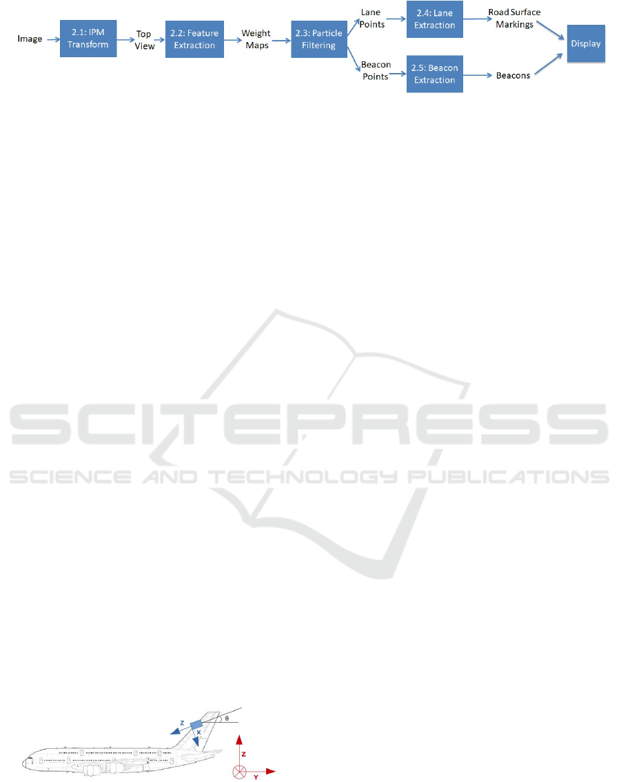
Figure 1: Functions for interpretation of airport scenes.

aircraft vertical ﬁn. Different observation maps are

then created from this top view, and used by a particle

ﬁlter for the detection of lines. The use of the particle

ﬁlter is motivated by the need to implement a proba-

bilistic method instead of a deterministic one, as we

work on weak models. Clusters of points are collected

from the particle ﬁlter, arranged and merged to deter-

mine the line equations by polygonal approximation.

Other elements such as beacons are detected on the

taxyway in the same way, and added to the detected

lines to produce an augmented reality view of the tax-

iway.

The next section describes different functions in-

tegrated in our scene interpretation module. Results

are presented in the section 3, while contributions and

current works are summarized in the section 4.

2 METHODS

The different functions described in this section are

shown on Figure 1: they currently aim at building an

augmented view to be displayed in the cockpit; the

scene representation will be used later for alerting the

pilot if a risky situation is detected, or for autonomous

navigation of the aircraft on taxiways.

2.1 Inverse Perspective Mapping (IPM)

As presented in (Deng et al., 2013), the scene can be

presented, in the Euclidian space, either in the world

coordinate system or in any chosen image coordinate

system. We decided to use a top view transformation

by applying an Inverse Perspective Mapping to our

frame. The coordinate systems used are illustrated in

Figure 2.

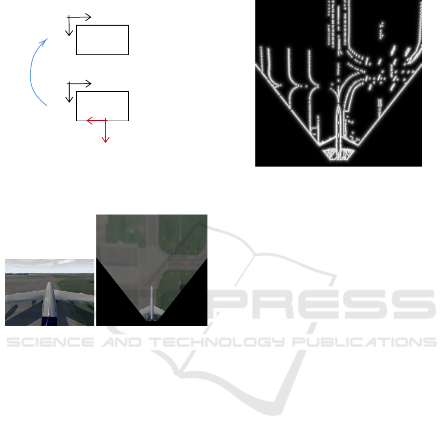
Figure 2: Representation of the camera coordinate system

(blue) and IPM coordinate system (red).

Providing that we deﬁne a point in the world coor-

dinate system (respectively in the image coordinate

system) by the following coordinates P

, Y

, Z

)

(respectively P

, Y

, Z

)), we will note any trans-

formation in the world to camera coordinate system

process P

W /C

, Y

W /C

, Z

W /C

). The expression of

a point in the camera coordinate system is expressed

in Equation 1.

= [R

].P

+t (1)

, R

and R

represent the rotation between the two

coordinate systems in the three dimensions while t is

the translation part of the movement. P

can also be

deﬁned as in Equation 2

= [X

W /C

].P

+ 0

W /C

(2)

The homography H needed to change from the world

coordinate system to the image coordinate system can

be found in Equation 3. As we project the image on

the ground to create a top view, the Z

W /C

is not taken

into account. The homography used in our algorithm

can be found in Equation 4, where K is the intrinsic

matrix of the camera, D is the height of the camera

in relation to the ground and θ correspond to the tilt

value of the camera.

H = K.[X

W /C

] (3)

H = K.





−1 0 x

0 sin(θ) D.cos(θ)

0 −cos(θ) D.sin(θ)





(4)

To compute an IPM image adapted to our speciﬁcati-

ons, we perform a discretization of the image where

the dimensions of one cell are deﬁned as (δX, δY ).

This permits to describe the coordinate (i, j) of each

pixel in the IPM image in relation to its (X ,Y ) coor-

dinates in the image coordinate system. Equation 5

links the (i, j) and (X ,Y ) coordinates, where D

and

are the size of the IPM frame. The intensity of the

(i, j) cell is interpolated from the value of the (u, v)

cell in the image. The link between the (i, j) and

(u,v) coordinate is despicted in Equation 6. The Fi-

gure 3 exposes the IPM process. Results of the IPM

are presented in Figure 4. All the following image tre-

atments will be applied to the resulting image shown

in Figure 4(b).













0 1/∆Y D

−1/∆X 0 D

0 0 1













(5)

VISAPP 2019 - 14th International Conference on Computer Vision Theory and Applications

518

IPM image

Normal image

Figure 3: Creation of IPM frame from camera frame.









= H.









(6)

(a) (b)

Figure 4: (a) Original image, (b) IPM transformation.

2.2 Weighted Maps Computation

The transformed IPM image is used to create several

maps. The goal of these maps is to compute a weight

for each pixel before launching a particle ﬁlter on the

IPM image, for lane detection. The weight of a pixel

will increase as it is closer to the reference color of the

object to detect and its belonging to a detected border

of the object.

2.2.1 Edge Map Computation

Our algorithm uses two types of edge maps. One is

used to detect any border in the image whereas the

other is mainly based on the lane analysis. Combined,

they offer varied information.

The ﬁrst map is created by using the Sobel gra-

dient on the image intensity. The IPM image obtained

in Figure 4(b) is converted into a grayscale image and

a Sobel gradient is performed on the created image.

An exponential treatment is then applied to the re-

sult values in order to increase the contrast between

Figure 5: Edge map - Sobel Gradient.

black and white pixels. Figure 5 is an example of the

provided map where the blurry effect is created by

our exponentional treatment. The exponential para-

meters are chosen with regards to our data to express

the noise in the measurement and conﬁdence in the

measurement. The second edge map is based on the

model of a lane and a method proposed by (Bertozzi

and Broggi, 1998). In the aviation ﬁeld, speciﬁcations

are numerous and common to all airports. The sizes

of the lanes that can be found in an airport are regu-

lated. We use the knowledge of the lane size for this

edge detection. The IPM frame is ﬁrst converted in

the HSV (Hue, Saturation, Value) color-space, where

we select the saturation channel. The yellow color of

the lanes becomes much more expressive in this re-

presentation. Based on the knowledge of the road,

our algorithm skims the resulting image of the satu-

ration channel in order to create a binary version of

the image. Each pixel is compared to its left and right

neighbors, in terms of saturation value and a threshold

is ﬁxed to discriminate the pixels belonging to a lane

from the others. Once this binarization is computed,

we apply a distance transform, based on the algorithm

described by (Felzenszwalb and Huttenlocher, 2012)

and implemented in OpenCV, to the image obtained.

The result of this treatement is shown in Figure 6.

The map created thanks to the Sobel gradient ena-

bles our algorithm to detect geographical informati-

ons such as borders between the tarmac and the grass

or beacons. It can help to create a model of the scene

and ﬁlter false positive detections. The second map

is focused on the known size of the main lane to fol-

low in an airport and reduce the number of borders

to examine. To detect only a lane, we will use the

second map whereas the beacons and tarmac delimi-

tations are computed with the ﬁrst map.

Using the Sobel Gradient map combined with the

Lane Detection and Scene Interpretation by Particle Filter in Airport Areas

519

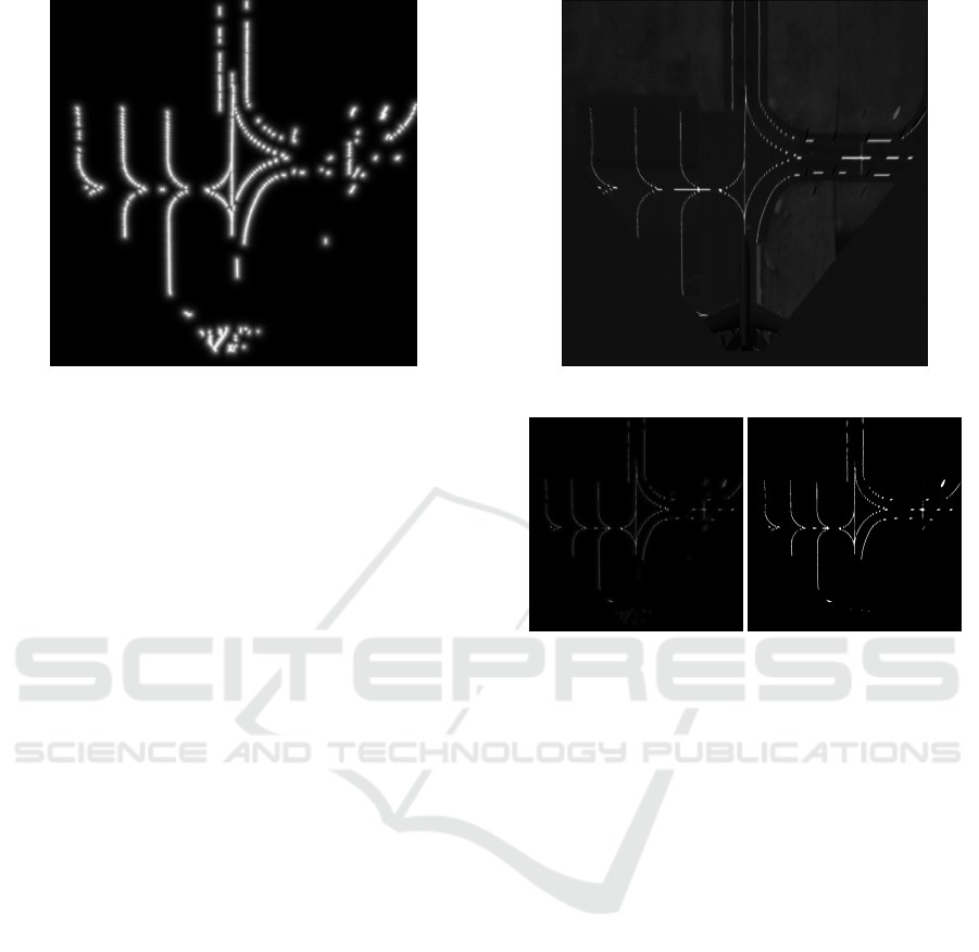
Figure 6: Edge map - Lane model.

second map could be efﬁcient for double checking as

the size of the lane can vary with partial occlusion

or curvy parts but the combination of the two maps

increase the computation time. We know that when

the lane becomes curvy, its apparent size in the IPM

image can be reduced and the lane might not be de-

tected by our algorithm. This is why we apply tre-

atments to the second map, to add noise in order to

simulate our conﬁdence in the measurement and in-

crease the detection rate.

2.2.2 Color Map Computation

The color of the various lanes that can be encounte-

red are regulated and deﬁned in speciﬁc range of yel-

low and white. We can use these speciﬁcations in our

model, to create a map of similarity between the co-

lor of a pixel and the reference color. To ensure that

the algorithm is more robust to wheather phenome-

nons such as shading, we compute the color map in

the LAB color-space. A patch of reference color is

deﬁned in the LAB color-space and our algorithm ap-

plies a convolution between this patch of the reference

color and the color IPM image (see Figure 4(b)) in or-

der to determine a distance between the two patches

of pixels, based on the A and B channels. Figure 7

shows the resulting color map.

2.2.3 Global maps computation

We combine the Edge and Color maps deﬁned above

to create a measure map. A value is attributed to

each pixel and represents the multiplication of a color

weight by the edge weight, computed thanks to the

two previous maps. A speciﬁc exponential treatment

is applied to the color and edge weights to increase the

contrast between a pixel belonging to a lane and the

others. We also create a binarized version of this map

Figure 7: Color map.

(a) (b)

Figure 8: (a) Weights map, (b) Binarized map.

used for the particle initialization while the weights

will be used for the particle survival estimation. The

results are presented in Figure 8, where it can be seen

that most of the additional noise brought by the edge

map is ﬁltered by the use of a combination of the two

maps, which increase the accuracy of the particle ﬁl-

ter and reduce the computation time.

2.3 Particle Filter

2.3.1 Particle Initialization

As explained in the introduction, we decided to use

a particle ﬁlter for the lane detection, using the

bootstrap ﬁlter or Sequential Importance Resampling

(SIR). The Figure 9 represents its operation. We will

note the state variable x

a random variable descri-

bing the state of a system at time t, y

a random

variable describing the sensor measurements at time

t, w

a variable describing the computed correction

of the predictions (importance weight) and q(x

0:t−1

0:t

) the proposal distribution. The particle ﬁl-

ter approximates the probable distribution of X

with

a set of samples, or particles noted p(x

0:t

| y

1:t

) com-

puted with

(i)

0:t

(i)

0:t

,i = 1..n

. Particles are upda-

VISAPP 2019 - 14th International Conference on Computer Vision Theory and Applications

520

Initialization Prediction

Correction



, ...x



Initial state :

(i)

∼ q



| x

(i)

0:t −1

0:t



ˆw

(i)

= w

(i)

t−1

∗ p



| x

(i)



(i)

ˆw

(i)

∑

j=1

ˆw

(i)

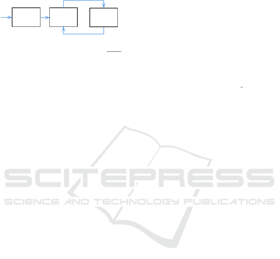
Figure 9: Principle of the particle ﬁlter.

ted through a series of predictions based on the prior

knowledge of the system and corrections of these pre-

dictions based on the sensor measurements. The esti-

mation of the current state variable ˆx

is selected with

the argmax function.

The initialization is done by scanning the global

map row by row, from bottom to top, until white

pixels are detected, these pixels represent the proba-

ble starting point of a lane. The ﬁrst line composed

of white pixels will be used as the initialization. Any

group of connected white pixels is deﬁned as a seg-

ment on which we randomly scatter a deﬁned number

of particles.

2.3.2 Particle Correction and Future Prediction

The particle ﬁlter implemented in our algorithm scans

the image every n rows, where n has been deﬁned to

be small enough to detect possible new starts of la-

nes and big enough to reduce the computational time.

At initialization, these particles are associated to a

weight given by the global map. The weights are used

at time t > t

to give higher importance to most pro-

bable particles, thus resulting in better prediction for

future particles through multinomial resampling. The

weights of the different particles are normalized and

create a cumulative weights scale. Random values be-

tween 0 and 1 are computed and represented in this

scale where they are matched to speciﬁc particles.

To predict new particules, we only use, as past

positions, the positions of the particles related to the

random values. The new particles will follow a Gaus-

sian distribution centered around the past particle.

2.3.3 Cluster Mergings and Separations

As we said before, the airport areas are difﬁcult to

model because they can easily vary. While the parti-

cle ﬁlter scans the image row after row, new lanes can

appear, old lanes can disappear and several lanes can

merge to form only one remaining lane. It is also pos-

sible that false positives trigger new lanes detections.

The initialization of particle clusters for new detected

lanes at time t and the prediction of future particles

for already existing clusters are done before launching

the t + 1 step. To manage the cases where a lane can

disappear or when a false positive has created a sus-

picion of lane, we implemented several thresholds. A

survival likelihood is computed for each particle, with

regards to its weight and the weights of the other parti-

cles, such as in Equation 7 where w

is the normalized

weight, n is the number of particles and p

is the sur-

vival likelihood. Once several particles have reached

a determined value of survival likelihood, the cluster

of particles is terminated.

(

1, i f w

≥

n ∗ w

, otherwise

(7)

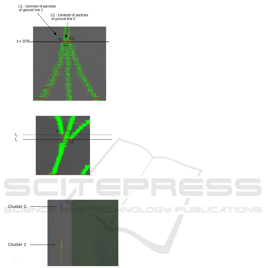
In case of merging of lanes or separation of a detected

lane in multiple lanes, we decided to study the ba-

rycenter of each cluster of particles. Based on their

proximity, our algorithm either merges the clusters in

one or creates new clusters for new detected lanes.

An illustration of this cases can be found in Figure 10

where the green pixels represent particles with high

survival likelihood while red pixels represent particles

with low survival likelihood. It also shows as new la-

nes are tracked and clusters are merged.

2.4 Line Extraction

2.4.1 Polygonal Approximation

Once the particle ﬁlter processing of the image is ﬁ-

nished, the algorithm output is a list of all the crea-

ted clusters and the positions of its particles at each

iteration of the particle ﬁlter. We select the most pro-

minent particle for each iteration based on the parti-

cle weight. We then choose to approximate the de-

tected lanes by afﬁne equations. As the clusters can

sometime include curves, we perform a polygonal ap-

proximation. This increases the number of clusters

but the approximated lanes for the cluster positions

are more accurate. As the lanes in the tarmac will not

be too curvy, we can use this method without increa-

sing the computational time.

2.4.2 Line Fitting and Cluster Merging

Most of the time, we can see that a unique lane can be

separated in multiple clusters by the previous steps.

It also happens when there is a crossing in the image,

where a straight lane will separate in two and reappear

few meters ahead. As we need to give useful infor-

mation to the pilots, we decided to recreate this lanes

by merging the clusters. Figure 11 is an example of

Lane Detection and Scene Interpretation by Particle Filter in Airport Areas

521

(a)

(b)

Figure 10: (a) Fusion of clusters, (b) New lane tracking.

Figure 11: Clusters to be merged together.

two clusters to be merged together to form one lane.

For each cluster of positions, we use a line ﬁtting

algorithm. Lines can either be vertical or horizontal.

To be able to compute the cluster line equation, we

differenciate these two cases. Once lines have been

computed for each cluster, we compare them between

each other in order to merge similar clusters and re-

create the observed lanes in the image.

2.5 Beacon Extraction

The main goal of our algorithm is to perform scene

analysis and lane detection. In the sections 2.2

and 2.3, we deﬁned the method for the lane detection

but it can also be applied for beacon detection or tar-

mac limits detection. For the lane detection, we used

an edge map based on the model of a vertical straight

lane. In order to detect the horizontal lanes, we per-

form a transposition on the image before launching

our algorithm again. The results of the two iterations

are then mixed together. The process is also simi-

lar for beacons detection, for which we use the Sobel

edge map and a speciﬁc color map. As we use the

IPM view, the beacons are deformed and can be seen

as little blue stripes. Those are detected by our al-

gorithm, from which we select the ﬁrst position, as it

represents the real position of the beacon.

3 RESULTS

In order to illustrate the results of our algorithm, we

simulated a case of line intersection, as we can see in

Figure 4(b), which is a case that can commonly occur

in airport areas.

The airplane model used for this simulation

is a A380 and the camera, which resolution is

1280pX960p and horizontal ﬁeld of view is 80 de-

grees, is mounted on its ﬁn at a distance D of 19,5

meters above the ground and an angle θ of 20 de-

grees. Our goal is to perform scene analysis to im-

prove pilots comprehension of the environment. Our

speciﬁcations is to analyse the scene up to 350 meters

ahead. For our algorithms, the image is represented

by an IPM view of resolution 1400pX14OOp where

each pixel represents an area of 25cmX25cm.

Figure 12 gives an overall view of the algorithm

results. In Figure 12(a) the green pixels represent

the estimation of the beacon position. Figure 12(b)

shows the results of the particle ﬁlter on the vertical

lines, with red points representing the particles with

low survival likelihood, where lines estimations are

highlighted in green in Figure 12(c). Figure 12(d)

and 12(e) follow the same process but on the trans-

posed IPM image.

To produce an image which could be easily used

by pilots, we return to the original view by performing

an inverse homography to highlight the detected lanes

and beacons in the real image. The result is shown in

Figure 13, where Figure 13(a) shows the combination

of the clusters detected in Figure 12(b) and 12(d).

The estimation of the lines positions is quite accu-

rate. The positions of the beacons, colored in red in

Figure 13(b) are nearly all matching the original bea-

con positions. However, our algorithm does not pre-

cisely detect the curve part of the taxiway lanes. Any

curved part brings noise to the lane detection because

VISAPP 2019 - 14th International Conference on Computer Vision Theory and Applications

522

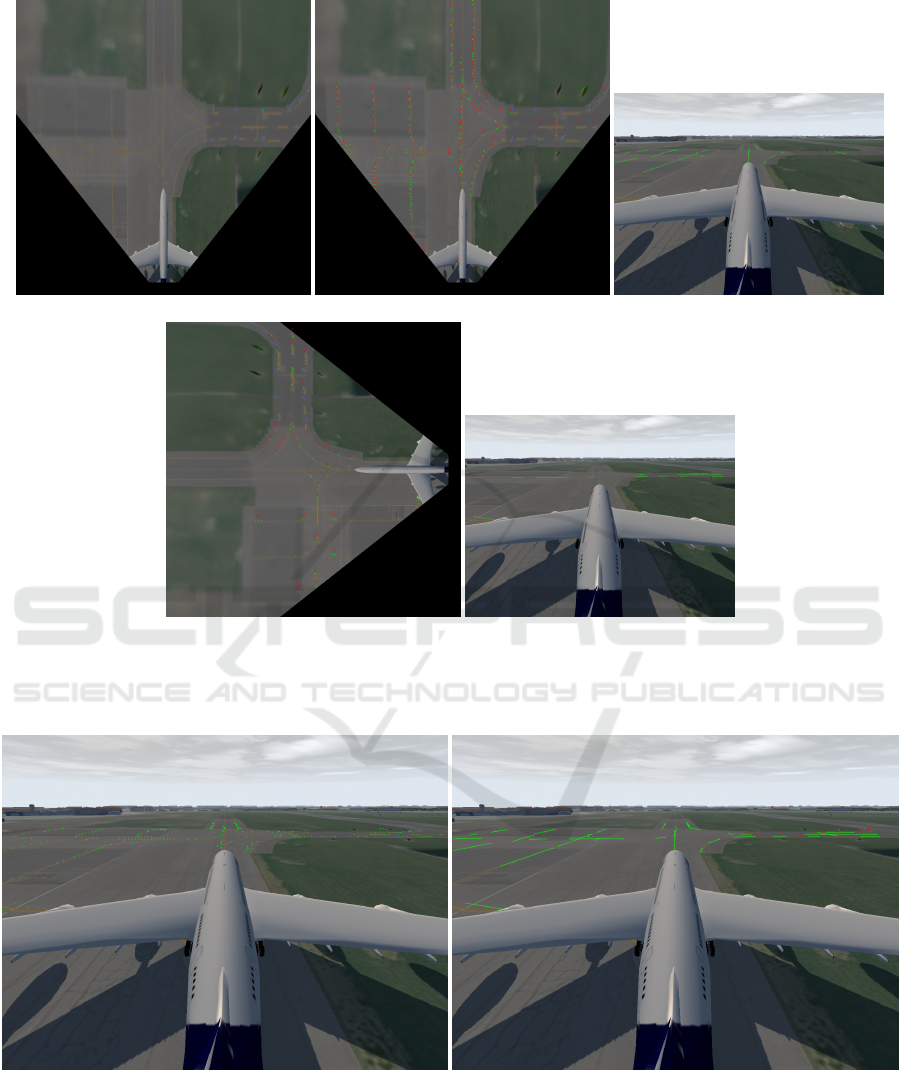
(a) (b) (c)

(d) (e)

Figure 12: (a) Detected beacons based on the original image, (b) Position of clusters from the particle ﬁlter based on the

original image, (c) Detected lines based on the original image, (d) Position of clusters from the particle ﬁlter based on the

transposed image, (e) Detected lines based on the transposed image.

(a) (b)

Figure 13: (a) Result of the combined position of clusters, (b) Result of the combined lines (green) and beacons (red).

our lane detection algorithm is based on an edge map

established by the lane model. On curved parts, the

lane model is modiﬁed and not accurately represen-

ted in the resulting edge map. Merging the two edge

maps in one with the same operation used to create

the global weights map could improve our algorithm

accuracy on curved parts without signiﬁcantly increa-

sing the computation time.

Lane Detection and Scene Interpretation by Particle Filter in Airport Areas

523

4 CONCLUSIONS AND

PERSPECTIVES

In this paper, we presented an accurate algorithm for

scene analysis and lane detection in an airport taxi-

way, based on an IPM transformation and a particle

ﬁlter. For the moment, the algorithm is based on a

straight lane model. For curved parts, as the lane mo-

del changes, we will need to explore new models, in

order to detect any type of lanes in the scene and give

a more detailed view to the pilots. Extra tuning of

the road size threshold based on the modelling of the

size decrease in curved parts would greatly increase

the lane detection.

By now, images used for our algorithm validation

are produced by a simulator. They are modelised at

daytime, with clear weather conditions. Our objective

is to generalize our algorithm to other weather con-

ditions such as night time, rainy or foggy days. To

achieve this, we plan to increase our dataset by com-

bining information from RGB camera and IR camera.

As the simulation tool can be tuned to match our ca-

mera, we can work on images similar to real ones.

Our future goal is to use the combination of lanes

and beacons, with the help of other scene elements

such as the tarmac limits and panels on the side of

the tarmac for example, to implement a line tracking

algorithm. This algorithm will enable us to perform

egomotion estimation. This information can then be

used in an object detection algorithm also based on

an IPM transformation, which goal is to detect ob-

jects combining the egomotion estimation and images

at time t and t −1.

For now, our algorithm is not optimized and is

launched on a basic computer, with a computation

time of few seconds for lines, beacons and tarmac de-

tection for one image. In the future, we plan to opti-

mize the code and implement it on a dedicated archi-

tecture including multi-cores CPU, GPU and FPGA.

ACKNOWLEDGEMENTS

We would like to thank the OKTAL-SE company for

providing a simulation tool which provides images,

close to real images, for testing the method.

REFERENCES

Asif, M., Arshad, M. R., Zia, M. Y. I., and Yahya, A. I.

(2007). An implementation of active contour and kal-

man ﬁlter for road tracking. International Journal of

Applied Mathematics, 37(2):71–77.

Bertozzi, M. and Broggi, A. (1998). Gold: a parallel real-

time stereo vision system for generic obstacle and lane

detection. IEEE transactions on image processing :

a publication of the IEEE Signal Processing Society,

7(1):62–81.

Chapuis, R., Potelle, A., Brame, J., and Chausse, F.

(1995). Real-time vehicle trajectory supervision on

the highway. The International Journal of Robotics

Research, 14(6):531–542.

Deng, J., Kim, J., Sin, H., and Han, Y. (2013). Fast lane

detection based on the b-spline ﬁtting. International

Journal of Research in Engineering and Technology,

2(4):134137.

Felzenszwalb, P. F. and Huttenlocher, D. P. (2012). Distance

transforms of sampled functions. Theory of Compu-

ting, 8:415–428.

Hota, R. N., Syed, S., B, S., and Radhakrishna, P. (2009).

A simple and efﬁcient lane detection using clustering

and weighted regression. In 15th International Confe-

rence on Management of Data, COMAD.

Jiang, R., Klette, R., Vaudrey, T., and Wang, S. (2010).

Lane detection and tracking using a new lane model

and distance transform. Machine Vision and Applica-

tions, 22:721–737.

Lipski, C., Scholz, B., Berger, K., Linz, C., Stich, T., and

Magnor, M. (2008). A fast and robust approach to

lane marking detection and lane tracking. 2008 IEEE

Southwest Symposium on Image Analysis and Inter-

pretation, pages 57–60.

Loose, H. and Franke, U. (2010). B-spline-based road mo-

del for 3d lane recognition. 13th International IEEE

Conference on Intelligent Transportation Systems, pa-

ges 91–98.

Sehestedt, S., Kodagoda, S., Alempijevic, A., and Dissana-

yake, G. (2007). Robust lane detection in urban envi-

ronments. 2007 IEEE/RSJ Int. Conference on Intelli-

gent Robots and Systems, pages 123–128.

Sun, T.-Y., Tsai, S.-J., and Chan, V. (2006). Hsi color mo-

del based lane-marking detection. 2006 IEEE Intelli-

gent Transportation Systems Conference, pages 1168–

1172.

Theuma, K. and Mangion, D. Z. (2015). An image pro-

cessing algorithm for ground navigation of aircraft.

In Bordeneuve-Guib

e, J., Drouin, A., and Roos, C.,

editors, Advances in Aerospace Guidance, Navigation

and Control, pages 381–399, Cham. Springer Interna-

tional Publishing.

Tomas, B., Ondrej, K., and Ondrej, P. (2017). Methods and

systems for providing taxiway stop bar information to

an aircrew.

VISAPP 2019 - 14th International Conference on Computer Vision Theory and Applications

524