cudaIFT: 180x Faster Image Foresting Transform for Waterpixel

Estimation using CUDA

Henrique M. Gonc¸alves

1,3

, Gustavo J. Q. de Vasconcelos

1,3

, Paola R. R. Rangel

1,4

, Murilo Carvalho

Nathaly L. Archilha

and Thiago V. Spina

1,∗

Brazilian Synchrotron Light Laboratory, Brazilian Center for Research in Energy and Materials, Campinas, SP, Brazil

Brazilian Bioscences National Laboratory, Brazilian Center for Research in Energy and Materials, Campinas, SP, Brazil

Institute of Computing, University of Campinas, Campinas, SP, Brazil

Institute of Geosciences, University of Campinas, Campinas, SP, Brazil

Keywords:

Image Foresting Transform, GPU, Watershed, Image Segmentation, Superpixels.

Abstract:

We propose a GPU-based version of the Image Foresting Transform by Seed Competition (IFT-SC) operator

and instantiate it to produce compact watershed-based superpixels (Waterpixels). Superpixels are usually

applied as a pre-processing step to reduce the amount of processed data to perform object segmentation.

However, recent advances in image acquisition techniques can easily produce 3D images with billions of

voxels in roughly 1 second, making the time necessary to compute Waterpixels using the CPU-version of the

IFT-SC quickly escalate. We aim to address this fundamental issue, since the efﬁciency of the entire object

segmentation methodology may be hindered by the initial process of estimating superpixels. We demonstrate

that our CUDA-based version of the sequential IFT-SC operator can speed up computation by a factor of up to

180x for 2D images, with consistent optimum-path forests without requiring additional CPU post-processing.

1 INTRODUCTION

Image segmentation is a crucial task for many appli-

cations in computer vision and image analysis. It is a

challenging process given the wide variety of objects

that may be depicted in different imaging modalities

(e.g., medical, natural, and geological images). To ad-

dress this issue, several methods rely on performing a

ﬁrst level of image segmentation by generating super-

pixels. Superpixels divide an image into homogene-

ous regions such that adjacent pixels with similar in-

tensities/colors are assigned to a same region. Seman-

tic objects are then usually comprised by one or more

of those regions. The object segmentation methods

aim to classify and/or merge the superpixels to per-

form the ﬁnal segmentation and separate the desired

objects of interest (Stegmaier et al., 2016; Stegmaier

et al., 2018; Rauber et al., 2013).

Superpixel estimation is important because (i) it

permits image segmentation methods to aggregate lo-

cal contextual information about the different regions

of the objects (an object may contain very dissimi-

lar parts), and because (ii) it may signiﬁcantly reduce

Corresponding author

the computational effort for segmentation, since the

amount of estimated superpixels is usually far lower

than the number of pixels in the image. Hence, se-

veral methods have been proposed to extract super-

pixels from an image (Achanta et al., 2012; Lotufo

et al., 2002; Alexandre et al., 2015; Machairas et al.,

2015; Vargas-Mu

noz et al., 2018; Felzenszwalb and

Huttenlocher, 2004).

Superpixel extraction methods ought to strike

a balance between achieving high boundary recall

and obtaining compact regions (Vargas-Mu

noz et al.,

2018). The former evaluates how the superpixels cap-

ture the borders of the existing objects in the image,

while the latter is concerned with producing regions

with shape as regular as possible. Compactness is im-

portant because regular shaped regions facilitate the

posterior extraction of features for object segmenta-

tion. Methods such as the Simple Linear Iterative

Clustering (Achanta et al., 2012) (SLIC) have been

proposed with compactness in mind, to counterba-

lance approaches that produce irregular regions such

as the watershed transform (Falc

ao et al., 2004; Roer-

dink and Meijster, 2000). The latter, however, can

usually achieve higher boundary recall at the expense

of region compactness.

Gonçalves, H., Q. de Vasconcelos, G., Rangel, P., Carvalho, M., Archilha, N. and Spina, T.

cudaIFT: 180x Faster Image Foresting Transform for Waterpixel Estimation using CUDA.

DOI: 10.5220/0007402703950404

In Proceedings of the 14th International Joint Conference on Computer Vision, Imaging and Computer Graphics Theory and Applications (VISIGRAPP 2019), pages 395-404

ISBN: 978-989-758-354-4

395

More recently, some authors have devised hybrid

methods that combine the characteristics of the su-

perpixel estimation by the watershed transform and

SLIC (Achanta et al., 2012) to leverage their comple-

mentary properties, such as the IFT-SLIC (Alexandre

et al., 2015), the Compact Watershed (Neubert and

Protzel, 2014), and the Waterpixels (Machairas et al.,

2015) approaches. All of the aforementioned techni-

ques rely on variants of the seeded watershed trans-

form, which can be efﬁciently implemented by using

the Image Foresting Transform (Falc

ao et al., 2004)

(IFT), a tool for the design of image processing and

pattern recognition operators based on optimum con-

nectivity. The IFT works by promoting a competition

among candidate pixels selected as the representati-

ves of the superpixels, henceforth denoted as seeds,

to conquer the remaining pixels of the image. The

resulting regions can be tuned in the aforementioned

hybrid approaches to exhibit either the compactness

of SLIC superpixels or the superior boundary adhe-

rence of the watershed transform.

In this work, we propose a GPU-based version of

the IFT by optimum seed competition operator (IFT-

SC) and instantiate it to produce Waterpixels (Fig. 1).

We aim to address one of the key issues overlooked by

the previously stated hybrid approaches: superpixel

estimation must be performed in timely fashion. Alt-

hough linear-time sequential implementations for the

IFT-SC exist (Falc

ao et al., 2004), the required com-

putational time can quickly escalate with the incre-

ase in the size of the image. This is particularly true

for 3D images, since recent image acquisition techni-

ques (Costa et al., 2017) can easily produce images

with billions of voxels in a few seconds (1500

voxel

images in about 1 − 5s). Hence, even though the di-

mensionality of the object segmentation problem is

reduced when using superpixels, the efﬁciency of the

entire approach can be hindered by the initial process

of estimating them (Rauber et al., 2013).

The IFT-SC can be understood by making an ana-

logy with the ordered formation of communities. Con-

sider a population in which each individual has the

desire of forming a community. Some natural born

leaders (seeds) begin the process by offering a re-

ward to their acquaintances to become part of their

community. If the reward is higher than the acquain-

tance’s desire of forming his/her own community,

or the acquaintance’s current reward if it is already

part of one, the acquaintance accepts the invitation

and changes communities. The communities grow

through their members, who start offering rewards

that are not higher than their own reward/desire. This

process continues following the non-increasing or-

der of reward/desire, until each individual is part of

(a) Input image (b) Seed set S, with σ = 20

daIFT

Figure 1: Waterpixel computation on a 2D slice of a CT

image of dolomite rock sample, using the cudaIFT pa-

rallel algorithm with regularly spaced seeds (σ = 20 and

k = 1000, see Equations 1-2).

the community that offered the highest reward. In

superpixel estimation, the population represents the

image, the individuals are the pixels, and each com-

puted community corresponds to a superpixel rooted

at the seed pixel (community leader) selected as its

representative.

To implement the IFT-SC in GPU, we allow each

individual of the population to begin conquering new

individuals as soon as they become part of a growing

community. Hence, we allow parallel competition be-

tween communities to occur, even if the reward that

can be offered by their individuals is not yet opti-

mum. In other words, we do not require the order

of reward/desire to be respected. We then iterate the

competition a few times to ensure that the rewards are

as close to the expected optimum value as possible,

thereby leading to a parallel version of the IFT algo-

rithm. We have implemented our method using Nvi-

dia’s CUDA language and therefore name it cudaIFT.

cudaIFT is related to the parallel implementation

of the Relative Fuzzy Connectedness algorithms pro-

posed in (Wang et al., 2016; Zhuge et al., 2012).

Those works tend to either parallelize the execution

considering some order during optimum reward pro-

pagation (Zhuge et al., 2012), or heavily rely on glo-

bal GPU memory with costly access (Wang et al.,

2016). cudaIFT thus presents several important con-

tributions:

VISAPP 2019 - 14th International Conference on Computer Vision Theory and Applications

396

1. It considerably improves the usage of GPU by ma-

king better use of CUDA threads during competi-

tion;

2. It makes heavy use of shared block memory

instead of global GPU memory to increase throug-

hput;

3. It is a parallel version of the IFT-SC operator, and

therefore can be used in settings other than Water-

pixel estimation.

We validate cudaIFT for the estimation of Water-

pixels in 2D slices of a 3D Computed Tomography

image, against the linear-time implementation of the

sequential IFT algorithm (Falc

ao et al., 2004). cu-

daIFT computes accurate superpixels with consistent

optimum-path forest, without requiring further CPU

post-processing, while achieving speedups of up to

roughly 180x over the CPU version.

The next sections are organized as follows.

Section 2 presents an overview of background con-

cepts that are necessary to understand Waterpixel es-

timation and the IFT algorithm. Section 3 provides

the algorithmic details about the cudaIFT approach.

We present our experimental validation in Section 4

and draw our ﬁnal conclusions in Section 5.

2 BACKGROUND

Image segmentation provides high-level knowledge

about the content of the image, by representing the

objects of interest depicted in the image. An image

I : D

→ V ⊆ R

is a mapping function from the rec-

tangular image domain D

⊂ Z

to the m-dimensional

real domain, such that m scalars are assigned to each

pixel in p ∈ D

. In this work, we are interested in

grayscale images (m = 1) represented in two dimen-

sional space (d = 2), making the array index p repre-

sent matricial image coordinates as p = (x, y). The

goal of image segmentation is to assign a label L(p)

to each pixel p in an image I corresponding to one

out of c available objects of interest or the background

(L(p) = 0).

In the following, we brieﬂy describe some back-

ground concepts necessary to understand the super-

pixel estimation method named Waterpixels, and the

sequential Image Foresting Transform algorithm. For

simplicity, the aformentioned label assignment L(p)

shall refer to the computed c regions, with each re-

gion reprepresenting a superpixel.

2.1 Waterpixel Estimation

The Waterpixels approach was proposed in (Machai-

ras et al., 2015) (Fig. 1). In order to strike a balance

between compactness and boundary recall, the Water-

pixels method performs the watershed transform on a

specially crafted border image B, which takes into ac-

count the position of the seed pixels in a set S selected

on a regular grid with spacing of σ pixels (Fig. 1b).

Image B (Fig. 1c) combines the gradient magnitude

of the input image

∇I

and a distance map E from

the seed set S:

B(p) =

∇I (p)

+ kE(p), (1)

in which k is an application-dependent parameter that

controls the tradeoff between compactness and boun-

dary adherance, and E is computed as

E(p) =

min

q∈S

{d(p, q)}, (2)

with d(p, q) = ||p − q|| being the euclidean distance

between pixels p and q. If k is small in Eq. 1, the

watershed transform is forced to adhere to the origi-

nal boundaries of image I . When k → ∞, the wa-

tershed transform becomes a Voronoi tessellation. It

is worth noting that both the computation of the gra-

dient image ∇I and the seed distance map E can be

very efﬁciently done on the GPU using, in the former

case, the Sobel operator for instance. Hence, those

optimizations are not the focus of this paper.

2.2 The Image Foresting Transform

The Image Foresting Transform can be seen as ge-

neralization of Dijkstra’s single source shortest path

algorithm (Dijkstra, 1959) for multiple sources and a

greater variety of connectivity functions (Falc

ao et al.,

2004; Ciesielski et al., 2018). The IFT algorithm can

be used to implement operators such as the waters-

hed transform (IFT-SC (Falc

ao et al., 2004)), supervi-

sed (Papa et al., 2012) and unsupervised (Rocha et al.,

2009) pattern classiﬁers, among others (Miranda and

Mansilla, 2014).

The IFT interprets an image as graph, in which the

pixels are the nodes and spatially adjacent elements

are connected by an arc. The aforementioned ordered

community formation analogy is therefore cast into

a graph-partitioning problem (Fig. 2). We describe

next the main elements required for using the IFT for

watershed image segmentation.

2.2.1 Graphs from Images

Let G = (N , A, w) denote a weighted graph, in which

N is a set of elements taken as nodes and A ⊆ N ×N

cudaIFT: 180x Faster Image Foresting Transform for Waterpixel Estimation using CUDA

397

...

Circular

priority

queue

seeds

start

first cost level

second cost level

third cost level

Sequential IFT Algorithm

...

Figure 2: The Image Foresting Transform sequential algo-

rithm diagram, depicting the intermediate result of the com-

munity formation procedure. The color code indicates the

sequence in which the pixels will be evaluated, according to

the ﬁnal optimum path cost that they will have.

is a binary and non-reﬂexive adjacency relation be-

tween elements of N that form the arcs. We use

q ∈ A(p) or (p, q) ∈ A to indicate that a node q ∈ N

is adjacent to a node p ∈ N . Each arc (p, q) ∈ A is

given a ﬁxed weight w(p, q) that encodes the dissimi-

larity between adjacent nodes p, q ∈ N .

For a given graph G = (N , A, w), a path π

, q

, . . . , qi with terminus at a node q is simple

when it is a sequence of distinct and adjacent nodes.

A path π

= π

· hp, qi indicates the extension of a

path π

by an arc (p, q) and a path π

= hqi is said

trivial. A connectivity function f assigns to any path

in the graph a value f (π

). A path π

is optimum

if f (π

) ≤ f (τ

) for any other path τ

in G.

In this work, we are interested in the traditional

max

connectivity function:

max

(hqi) =



0 if q ∈ S,

+∞ otherwise

max

(π

· hp, qi) = max{ f

max

(π

), w(p, q)}.(3)

Function f

max

essentially propagates the maximum

edge weight along a path. By assigning initial con-

nectivity values of 0 to trivial paths of nodes q belon-

ging to a set of previously selected seed pixels S, we

ensure that the IFT will force the seeds to compete

among themselves to conquer the remaining nodes of

the graph N \ S . The IFT algorithm may consider

several types of connectivity functions (Miranda and

Mansilla, 2013; Miranda et al., 2012), although a pro-

found study about other functions is outside the scope

of this work.

2.2.2 Optimum Path Forest

Considering all possible paths with terminus at each

node q ∈ N , an optimum connectivity map V (q) is

created by

V (q) = min

∀π

in (N ,A,w)

{ f (π

)}. (4)

The IFT solves the minimization problem above

by computing an optimum-path forest — a function

P which contains no cycles and assigns to each node

q ∈ N either its predecessor node P(q) ∈ N in the

optimum path or a distinctive marker P(q) = nil 6∈ N ,

when hqi is optimum (i.e. q is said root of the forest).

In essence, pixels in the seed set S become the roots

of the forest due to the initialization of function f

max

in Eq. 3. We present next the sequential IFT algorithm

for solving the minimization problem of Eq. 4.

2.2.3 Sequential IFT Algorithm

Algorithm 1 presents the steps to compute the IFT

following the minimization of Eq. 4. It relies on a

priority queue Q to propagate optimum path costs in

orderly fashion on weighted graph G.

Algorithm 1.: Sequential IFT Algorithm.

INPUT: Graph G = (N , A, w) and connectivity function f .

OUTPUT: Optimum-path forest P, its connectivity value map V

and its root map R.

AUXILIARY: Priority queue Q and variable tmp.

1. For each q ∈ N , do

P(q) ← nil, and V (q) ← f

max

(hqi).

3. If V (q) 6= +∞, then insert q in Q.

4. While Q 6=

0, do

5. Remove p from Q such that V (p) is minimum.

6. For each q ∈ A(p), such that V(q) > V (p), do

7. Compute tmp ← f

max

(π

· hp, qi).

8. If tmp < V (q), then

9. If V (q) 6= +∞, then remove q from Q.

10. Set P(q) ← p, V(q) ← tmp.

11. Insert q in Q.

Steps 1–3 initialize maps for trivial paths. The mi-

nima of the initial map V compete with each other

and the ones in seed set S become roots of the fo-

rest. They are nodes with optimum trivial-path values,

which are inserted in queue Q. The main loop com-

putes an optimum path from the roots to every node p

in a non-decreasing order of path value (Steps 4–11).

At each iteration, a path of minimum value V (p) is

obtained in P when we remove its last pixel p from Q

(Step 5). Ties are broken in Q using ﬁrst-in-ﬁrst-out

policy. The remaining steps evaluate if the path that

reaches an adjacent pixel q through p is cheaper than

the current path with terminus q and update Q, V (q),

and P(q) accordingly.

Seeded watershed segmentation using the IFT al-

gorithm is known as the Image Foresting Transform

by Seed Competition (IFT-SC) operator. In this work,

VISAPP 2019 - 14th International Conference on Computer Vision Theory and Applications

398

it can be straightforwadly derived by considering a

graph G

= (N , A, w) with the nodes N = D

as the

entire domain of image I and a spatial connectivity

function A = A

connecting 4-adjacent pixels. To

ensure that Waterpixels are computed through IFT-

SC, the seed set S is selected as the superpixel seeds

and the arc weights of graph G

are assigned as

w(p, q) = B(q), both of which as previously deﬁned

in Section 2.1.

Since arc weights can be normalized to integer va-

lues ranging from {0, 1, . . . , K}, Dial’s bucket sorting-

based priority queue (Dial, 1969) is usually selected

as Q in Algorithm 1. Hence, for sparse graphs as in

the case of 4- or 8-connected image-graphs, the al-

gorithm’s complexity is O(K + N ), being essentially

linear for reasonable values of K.

3 THE cudaIFT ALGORITHM

The main challenge of the parallelization of Al-

gorithm 1 lies on the fact that the IFT computes

optimum-path costs in greedy fashion, starting from

the seeds and extending paths incrementally follo-

wing the order given by the priority queue. One pre-

viously adopted strategy for implementing the IFT al-

gorithm (Zhuge et al., 2012) on the GPU aimed to pa-

rallelize the competition respecting the sequence of a

virtual priority queue. In essence, competition would

take place simultaneously for pixels with the same

cost level. Hence, pixels with the same color in the

priority queue of Fig. 2 would be allowed to compete

to extend their optimum-path trees, as long as their

costs matched the current minimum value in the vir-

tual priority queue. This approach severely hinders

parallel competition, since the global sequence of the

queue is still respected.

cudaIFT instead aims to allow as much competi-

tion to take place as possible, by understanding that

competition occurs primarily between neighboring

regions of the image when computing superpixels.

Hence, cudaIFT divides the 2D image into a grid of

CUDA blocks, with one CUDA thread per pixel, and

keeps track of a pixel activation map. Each CUDA

thread veriﬁes if its pixel p is active in the map,

and then tries to conquer adjacent pixels q ∈ A(p).

Seeds are the ﬁrst nodes that are activated before any

competition takes place, and whenever a new pixel

is conquered it is immediately activated to continue

the optimum-path tree expansion process inside their

CUDA thread blocks (Fig. 3).

Due to intrablock synchronization capabilities, we

make use of atomic operations and allow competition

to occur only inside CUDA blocks ﬁrst. Then, we

resolve interblock propagation of optimum-path costs

(bottom of Fig. 3) and iterate the entire algorithm a

few times until no pixel is active. This is similar in

spirit to the approach in (Wang et al., 2016), although

with a number of advantages. First, we make heavy

use of the GPU’s shared memory to avoid expensive

global memory access. Second, we keep CUDA thre-

ads continuously checking if their pixel have been

activated, until all of the threads in their block have

concluded. Third, we compute not only the opti-

mum path cost map V , but also the predecessor map

P and label L consistently, with no need for posterior

CPU corrections. This is very important, since the

Relative Fuzzy Connectedness approach, parallelized

in (Wang et al., 2016), actually only requires a con-

sistent cost map V and therefore does not compute a

predecessor map P. We detail in the next sections the

cudaIFT algorithm.

3.1 Main Steps of cudaIFT

Algorithm 2 presents the main steps of cudaIFT. The

algorithm starts by initializing the proper connecti-

vity, predecessor, label, and activation maps by taking

into account the seeds in set S and the connectivity

function f

max

. The initialization kernel is a simple pa-

rallelization of a loop over the entire image and seed

set. Then, the intrablock competition kernel is invo-

ked to perform seed competition inside each CUDA

thread block. In order to propagate the optimum-path

costs between CUDA thread blocks, the appropriate

kernels are called three times in the loop of Step 4,

such that information is propagated between the cor-

ners of the blocks as pointed out in Fig. 3 and follo-

wing (Wang et al., 2016). Finally, all steps are iterated

M times to ensure that there are no more active pixels.

With each iteration, more and more pixels become

active thereby ensuring that the wavefront of optimum

path-costs is propagated even if a CUDA thread block

originally has no seeds. Hence, although we focus on

superpixel estimation cudaIFT can be used with an

arbitrary seed set S . It is important to note, however,

that we divide interblock competition into two similar

kernels for efﬁcient processing of larger images, since

rows and columns at the CUDA thread block borders

are evaluated separately.

Algorithm 2.: The cudaIFT Algorithm.

INPUT: Seed set S , optimum-path forest P, its connectivity va-

lue map V , and its label map L in global GPU memory.

Adjacency relation A , and connectivity function f

max

Number of iterations M.

OUTPUT: Optimum-path forest P, its connectivity value map V ,

and its label map L in CPU memory.

AUXILIARY: Activation map A.

cudaIFT: 180x Faster Image Foresting Transform for Waterpixel Estimation using CUDA

399

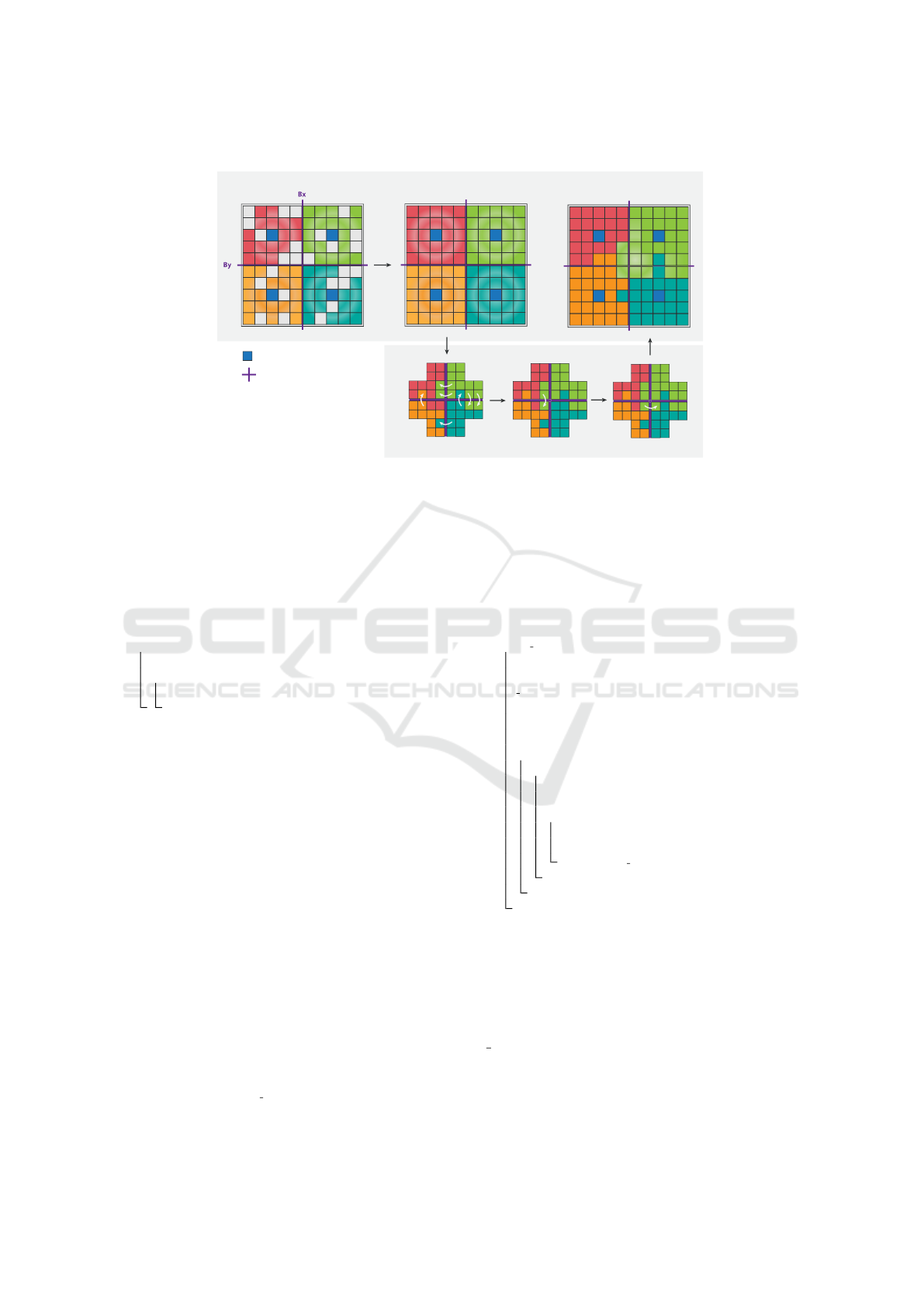
Interblock interactions

Intrablock competition

Proposed Parallel cudaIFT Algorithm

seeds

CUDA thread block division (Bx, By)

Final result

Temporary resultActive nodes

Figure 3: The proposed cudaIFT parallel algorithm diagram. Top: intrablock competition performed by active nodes in

shared memory, for small CUDA thread blocks (5x5 threads) and a single seed selected in each block. The left image depicts

active nodes during some step of the competition. The middle image presents the temporary result in shared memory after the

ﬁrst iteration of competition is done. The right image depicts the ﬁnal result, after some iterations of intrablock and interblock

competition are performed. Bottom: interblock competition performed by pixels on the boundary of CUDA blocks that were

activated during intrablock competition. The arrows indicate one node conquering another one from a different block. We

perform three interblock competition iterations for each intrablock competition to propagate information between the corners

of four adjacent blocks (a, b, c, d), as can be seen at the center of the three images.

1. Initialization-Kernel(V , L, P, A, A, S , f

max

2. For i ∈ {1, 2, . . . , M}do

3. Intrablock-Competition-Kernel(V , P, L, A, A, f

max

)

4. For j ∈ {1, 2, 3} do

5. Interblock-H-Competition-Kernel(V , P, L, A, A

, f

max

Interblock-V-Competition-Kernel(V , P, L, A, A

, f

max

7. Transfer maps L, V , and P to CPU/main memory.

3.2 Intrablock Competition

The intrablock competition kernel is run for each

pixel in the image domain p ∈ D

. CUDA threads

are spawned using a 32 × 32 block size with blocks

covering the entire image. Algorithm 3 presents the

intrablock competition kernel.

Algorithm 3.: Intrablock Competition Kernel.

INPUT: Global index of pixel p. Adjacency relation A . Activa-

tion map A. Optimum-path forest P, its connectivity va-

lue map V , and its label map L in global memory. Con-

nectivity function f

max

OUTPUT: Updated values in global memory of: optimum-path fo-

rest P, connectivity value map V, label map L, and acti-

vation map A.

AUXILIARY: Temporary variables active, tmp. Variables in shared

memory: activation map A

, cost map V

, predecessor

map P

, label map L

, mutex lock map K

, and termina-

tion variable s done .

1. Copy map values L(p),V (p), P(p) from global to shared memory.

2. syncthreads().

3. While s done 6= False, do

4. V

← V

(p).

5. L

← L

(p).

6. s done ← 1.

7. active ← A

(p).

8. Atomically set A

(p) ← False.

9. syncthreads().

10. If active = True, then

11. For each q ∈ A(p) do

12. Compute tmp ← f

max

(π

· hp, qi).

13. Try-Acquire-Lock(K

(q)).

14. If tmp < V

15. (V

(q) = tmp, P

(q) = p, L

(q) 6= L

), then

16. Set P

(q) ← p,V

(q) ← tmp.

17. A

(q) ← True, s done ← False.

18. Release-Lock(K

(q))

19. syncthreads().

20. syncthreads().

21. Copy map values L

(p),V

(p), P

(p) from shared to global memory.

First, the current label, cost, and predecessor maps

are copied to shared memory. Then, the kernel loops

while the pixels of the threads of the corresponding

CUDA block are active, given by shared variable

s done = True. While that is true, a snapshot of the

label and cost of the current pixel p is done, since

they may be altered by other threads during compe-

tition, and the pixel p is checked for activation. If

p is active (Step 10), then it will attempt to conquer

VISAPP 2019 - 14th International Conference on Computer Vision Theory and Applications

400

neighboring nodes q ∈ A(p). In order to conquer a

neighbor q, we need to ensure that only the current

thread is modifying the adjacent node’s connectivity,

label, and predecessor map values.

We have thus created a mutex procedure that es-

sentially tries to lock a map K

(q) in shared memory.

If successful, then the algorithm evaluates if the com-

puted cost value is lower than V

(q) and, if so, p is

able to conquer q (Step 14). However, since competi-

tion occurs in parallel and a voxel q is activated as

soon as it is reached, then sub-optimum path costs

may be propagated inadvertently. This becomes a

problem when ties in optimum costs exist, which may

lead to inconsistent label maps. Hence, we borrow

ideas from the differential IFT-SC operator (Falc

and Bergo, 2004), which is able to perform local cor-

rections after additions/removal of seed pixels, and

modify the test in Step 8 of the original IFT Algo-

rithm 1 to take into account ties in the path costs being

computed, as presented in Step 14 of Algorithm 3.

Since the mutex locking procedure is expensive, as

it involves a loop encompassing Steps 13-18 to ato-

mically verify if the state of the locking map K

(q) is

originally 0 and set it to 1 if true, in practice we repeat

the test of Step 14 before Step 13 to evaluate only can-

didate neighbors. Block thread synchronizations are

performed to ensure consistency of the competition.

3.3 Interblock Competition

The horizontal interblock competition procedure, gi-

ven in Algorithm 4, is quite similar to the intrablock

kernel. The main difference is that the competition is

executed only once for each pixel p on the boundary

of the CUDA thread blocks that divided the image

into a regular grid. Only the boundary pixels acti-

vated during intrablock competition are eligible for

interblock competition and to propagate information

to adjacent blocks. Note that the vertical competition

is essentially identical, what changes is that boundary

pixels on the columns are evaluated instead.

Algorithm 4.: Interblock Horizontal Competition Kernel.

INPUT: Global index of pixel p at the boundary of a CUDA

thread block from Algorithm 3. Adjacency relation in

the horizontal axis A

. Activation map A, optimum-path

forest P, connectivity value map V , label map L in global

memory. Mutex lock map K

in shared memory. Con-

nectivity function f

max

OUTPUT: Updated values in global memory of: optimum-path fo-

rest P, connectivity value map V, label map L, and acti-

vation map A.

AUXILIARY: Temporary variables active, tmp.

1. V

← V (p).

2. L

← L(p).

3. active ← A(p).

4. syncthreads().

5. If active = True, then

6. For each q ∈ A

(p) do

7. Try-Acquire-Lock(K

(q)).

8. Compute tmp ← f

max

(π

· hp, qi).

9. If tmp < V (q) or (V (q) = tmp, P(q) = p, L(q) 6= L

), then

10. Set P(q) ← p, L(q) ← L

, A(q) ← True.

11. Release-Lock(K

(q))

In the ﬁrst time that the intrablock competition

kernel is executed, all block boundary pixels are acti-

vated, but as iterations of the Algorithm 2 occur, this

number decreases until none is active. To this end, we

actually deactivate boundary pixels once Algorithm 4

is executed both horizontally and vertically after the

loop in Step 4 of Algorithm 2 is done, if the boundary

pixels are not activated during interblock competition.

4 EXPERIMENTAL RESULTS

We have conducted experiments comparing the se-

quential linear-time implementation of the IFT-SC al-

gorithm in C language, versus the cudaIFT algorithm

for estimation of Waterpixels. We have selected 2D

slices of a graycale 3D Computed Tomography image

of a carbonate rock sample to perform the compa-

rison, with original size of 1024

voxels. For each

slice, we carried out the comparison using 4 diffe-

rent seed spacing steps, namely σ = {5, 10, 20, 30},

to understand how seed sparseness affects computa-

tion. Parameter k in Eq. 1 was set to 1000 for all ex-

periments. The greater the value of σ the higher the

number of iterations (parameter M in Algorithm 2)

required for the result of the cudaIFT algorithm to

match the result of the sequential IFT-SC. Hence, we

executed up to M = 30 iterations but stopped as soon

as the computed optimum-path cost maps V for both

sequential and parallel algorithms matched. The sli-

ces were rescaled to encompass four different sizes

(1024

, 1536

, 2048

, and 4096

pixels), to evaluate

the speedup factor of the cudaIFT algorithm with in-

creasing amounts of pixels.

It is important to note that, due to the parallel na-

ture of cudaIFT, the forest map P and label map L may

differ from the result of the sequential IFT-SC due to

the asynchronous propagation of optimum paths. Ho-

wever, the differences in label and predecessor maps

only occur in zones where ties occur for the optimum-

path costs in map V. Therefore, in practice any result

in those regions corresponds to a valid optimum-path

forest P and the only thing that should truly match is

the optimum-path cost map V . Our veriﬁcation furt-

her ensured the consistency of the optimum-path cost,

cudaIFT: 180x Faster Image Foresting Transform for Waterpixel Estimation using CUDA

401

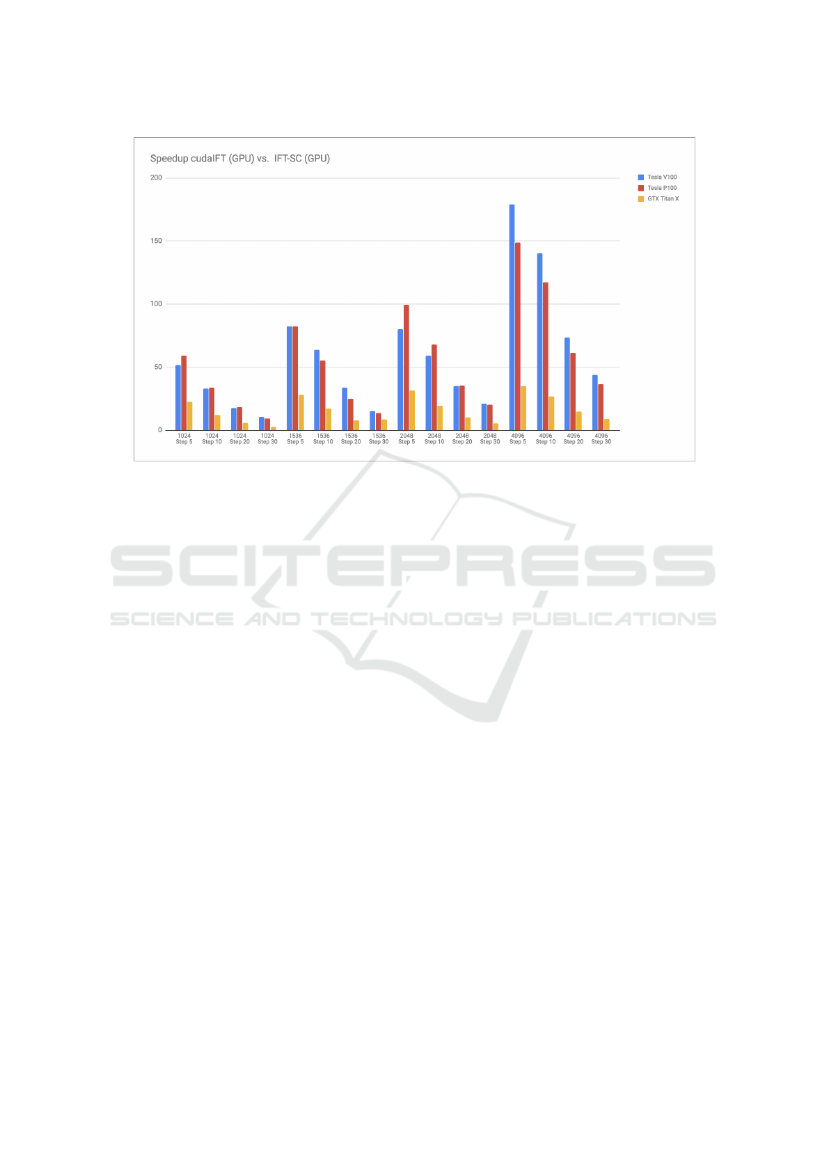
Figure 4: Average speedup factor for computing Waterpixels on 2D slices using cudaIFT vs. CPU IFT. Varying σ spacing

(steps) are considered to evaluate how seed sparseness affects the computational times. Different image sizes are also con-

sidered (|D

| = {1024, 1536, 2048, 4096}), for three different computer conﬁgurations with distinct GPUs (Nvidia Titan X,

Nvidia Tesla P100, and Nvidia Tesla V100).

forest, and label maps computed by cudaIFT.

We have executed the aforementioned experi-

ments 10 times for each slice and parameter setting,

in order to obtain statistics about the time measure-

ments. Our experiments were conducted using three

different machines, each with a distinct GPU and con-

ﬁguration to assess the algorithm in different environ-

ments. Our ﬁrst machine is a regular desktop with an

Intel Core i7-4790 CPU running at 3.60GHz, 8 GB of

memory RAM, Ubuntu 18.04 operating system, and

Nvidia GeForce GTX Titan X GPU with 3072 CUDA

Cores. The second is a server with an IBM Power 8

CPU running at 2.60GHz, 512 GB of memory RAM,

Ubuntu 18.04 OS, and Nvidia Tesla P100 GPU with

3584 CUDA Cores. The ﬁnal machine is a server with

an IBM Power 9 CPU running at 2.3GHz, 512 GB of

memory RAM, Ubuntu 18.04 OS, and Nvidia Tesla

V100 GPU with 5120 CUDA cores. CUDA 9.2 or

CUDA 10 were used in our experiments.

Figure 4 presents the average speedup factor for

the previously stated experiments, across all machine

conﬁgurations, without including CPU-GPU memory

transfer as the IBM Power servers possess NVLink

buses that could further increase the time difference

w.r.t. the used desktop. As expected, cudaIFT per-

forms signiﬁcantly better for larger images and smal-

ler step sizes. This occurs because smaller step sizes

decrease the amount of competition required to seg-

ment the images and generate superpixels. The server

running Nvidia Tesla V100 outperforms the others for

4096 × 4096 sized images, which can be explained

by the fact that Nvidia’s Volta architecture presents

superior atomic operations to the Pascal architecture

used for GTX Titan X and Tesla P100. In that case,

that conﬁguration may reach close to 180x speedup

for seeds with step size of σ = 5, and roughly 140x

speedup for σ = 10. Figure 5 depicts the average raw

computational times for the 4096 × 4096 sized ima-

ges for cudaIFT and IFT-SC in all three conﬁgurations

and four step sizes. It can be seen that IFT-SC takes

between 3.3s and 4.7s to execute, while the compu-

tational time for cudaIFT is always smaller than 0.5s,

reaching as low as 0.02s.

For other image sizes, we see a somewhat com-

petitive behavior between the P100 and V100 GPUs,

since the clock of the corresponding CPUs is slightly

lower for the latter. With respect to the Titan X GPU,

the others perform signiﬁcantly better since the Te-

sla P100 and Tesla V100 have compute capabilities

of 60 and 70, respectively, versus 52 for the GTX Ti-

tan X. This implies that the atomic operations for the

P100 is also superior, even though it has the same Pas-

cal architecture as the GTX Titan X and only a little

over 500 extra CUDA cores. Figure 6 conﬁrms the

aforementioned comparisons between GPUs and de-

monstrates that the cudaIFT runs usually from 2 − 5x

faster in Tesla P100 and Tesla V100 than GTX Titan

X. Similarly, Titan V100 is up to 1.8x faster than Te-

VISAPP 2019 - 14th International Conference on Computer Vision Theory and Applications

402

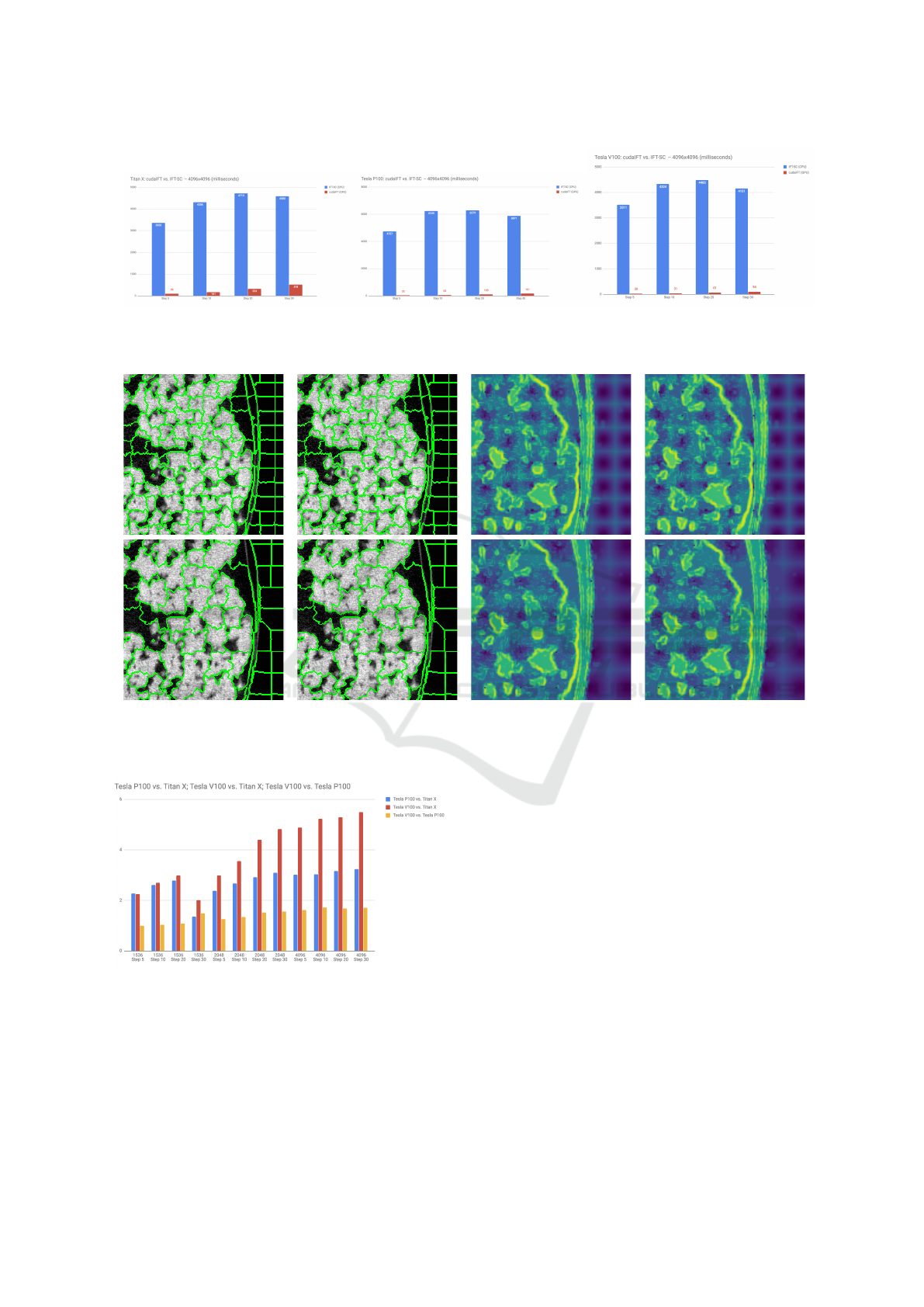
Figure 5: Raw computational times (in milliseconds) between cudaIFT and IFT-SC for image with size 4096 × 4096, for the

three different machines used in this work.

IFT-SC Label cudaIFT Label IFT-SC Cost cudaIFT Cost

Figure 7: Comparison between the label and cost maps obtained via cudaIFT and IFT-SC, for σ = 10 (top), σ = 20 (middle),

and σ = 30 (bottom). While the cost maps are identical, there are virtually no differences between the label maps.

Figure 6: Average speedup factor between GPUs for the

computation of cudaIFT.

sla P100. Figure 7 depicts some examples of cudaIFT

and IFT-SC results to demonstrate that the cost maps

are identical and that there are virtually no differences

in label assignment.

5 CONCLUSIONS

We have presented cudaIFT, a parallel version of the

IFT-SC operator using Nvidia’s CUDA language. cu-

daIFT is able to achieve up to roughly 180x speedup

over the sequential linear-time CPU implementation

of the IFT-SC operator, with perfectly consistent cal-

culations of the optimum-path forest. We have eva-

luated our algorithm to estimate Waterpixels in 2D

slices of 3D CT images of rock samples, and demon-

strated consistently superior results across three dif-

ferent machine conﬁgurations. In the future, we aim

to extend the method to work with 3D images and

non-planar image-graphs, and to automatically deter-

mine the number of iterations M. Our goal is to ens-

ure that large 3D and 4D images being acquired using

different imaging modalities with increasingly faster

speeds be segmented with the lowest possible proces-

sing time. We also intend to extend cudaIFT to handle

cudaIFT: 180x Faster Image Foresting Transform for Waterpixel Estimation using CUDA

403

other types of connectivity functions and evaluate it

with more general seed sets.

ACKNOWLEDGEMENTS

The authors would like to thank CNPEM, CAPES,

and the Serrapilheira Institute (Serra-1708-16161) for

the ﬁnancial support. The authors would like to thank

Dr. Tannaz Pak for the images used in this paper, as

well as Prof. Alexandre X. Falc

ao, Prof. Tiago J.

Carvalho, and Prof. H

elio Pedrini for the provided

insights and discussions.

REFERENCES

Achanta, R., Shaji, A., Smith, K., Lucchi, A., Fua, P., and

usstrunk, S. (2012). SLIC Superpixels Compared

to State-of-the-Art Superpixel Methods. IEEE Trans.

Pattern Anal. Mach. Intell., 34(11):2274–2282.

Alexandre, E. B., Chowdhury, A. S., Falc

ao, A. X., and Mi-

randa, P. A. V. (2015). IFT-SLIC: A general frame-

work for superpixel generation based on simple linear

iterative clustering and image foresting transform. In

SIBGRAPI, Salvador, Brazil.

Ciesielski, K. C., Falc

ao, A. X., and Miranda, P. A. V.

(2018). Path-value functions for which dijkstra’s al-

gorithm returns optimal mapping. J. Math. Imaging

Vis. Accepted.

Costa, G., Archilha, N. L., O’Dowd, F., and Vasconcelos,

G. (2017). Automation Solutions and Prototypes for

the X-Ray Tomography Beamline of Sirius, the New

Brazilian Synchrotron Light Source. In ICALEPCS,

pages 923–927, Barcelona, Spain. JACoW.

Dial, R. B. (1969). Algorithm 360: Shortest-path fo-

rest with topological ordering. Commun. ACM,

12(11):632–633.

Dijkstra, E. W. (1959). A note on two problems in connex-

ion with graphs. Numerische Mathematik, 1(1):269–

271.

Falc

ao, A. X. and Bergo, F. P. G. (2004). Interactive Vo-

lume Segmentation With Differential Image Foresting

Transforms. IEEE Trans. Med. Imag., 23(9):1100–

1108.

Falc

ao, A. X., Stolﬁ, J., and Lotufo, R. A. (2004). The

Image Foresting Transform: Theory, Algorithms, and

Applications. IEEE Trans. Pattern Anal. Mach. Intell.,

26(1):19–29.

Felzenszwalb, P. F. and Huttenlocher, D. P. (2004). Efﬁ-

cient Graph-Based Image Segmentation. Int. J. Com-

put. Vis., 59(2):167–181.

Lotufo, R. A., Falc

ao, A. X., and Zampirolli, F. A.

(2002). IFT-Watershed from gray-scale marker. In

SIBGRAPI, pages 146–152.

Machairas, V., Faessel, M., C

ardenas-Pe

na, D., Chabardes,

T., Walter, T., and Decenci

ere, E. (2015). Waterpixels.

IEEE Trans. Image Process., 24(11):3707–3716.

Miranda, P. and Mansilla, L. (2013). Oriented image fo-

resting transform segmentation by seed competition.

IEEE Trans. Image Process., PP(99):1–1.

Miranda, P. A. V., Falc

ao, A. X., and Spina, T. V. (2012).

Riverbed: A novel user-steered image segmentation

method based on optimum boundary tracking. IEEE

Trans. Image Process., 21(6):3042–3052.

Miranda, P. A. V. and Mansilla, L. A. C. (2014). Orien-

ted Image Foresting Transform Segmentation by Seed

Competition. IEEE Trans. Image Process., 23(1):389–

398.

Neubert, P. and Protzel, P. (2014). Compact watershed and

preemptive slic: On improving trade-offs of super-

pixel segmentation algorithms. In ICPR, pages 996–

1001, Stockholm, Sweden.

Papa, J. P., Falc

ao, A. X., de Albuquerque, V. H. C., and Ta-

vares, J. M. R. (2012). Efﬁcient supervised optimum-

path forest classiﬁcation for large datasets. Pattern

Recognition, 45(1):512 – 520.

Rauber, P. E., Spina, T. V., Rezende, P., and Falc

ao, A. X.

(2013). Interactive segmentation by image foresting

transform on superpixel graphs. In SIBGRAPI, Are-

quipa, Peru.

Rocha, L. M., Cappabianco, F. A. M., and Falc

ao, A. X.

(2009). Data clustering as an optimum-path forest

problem with applications in image analysis. Int J.

Imaging Syst. Technol., 19(2):50–68.

Roerdink, J. and Meijster, A. (2000). The watershed trans-

form: Deﬁnitions, algorithms and parallelization stra-

tegies. Fund. inform., 41:187–228.

Stegmaier, J., Amat, F., Lemon, W. B., McDole, K.,

Wan, Y., Teodoro, G., Mikut, R., and Keller, P. J.

(2016). Real-time three-dimensional cell segmenta-

tion in large-scale microscopy data of developing em-

bryos. Dev. Cell, 36(2):225–240.

Stegmaier, J., Spina, T. V., Falc

ao, A. X., Bartschat, A., Mi-

kut, R., Meyerowitz, E., and Cunha, A. (2018). Cell

segmentation in 3D microscopy images using super-

voxel merge-forests with CNN-based hypothesis se-

lection. In ISBI, Washington, USA.

Vargas-Mu

noz, J. E., Chowdhury, A. S., Barreto-Alexandre,

E., Galv

ao, F. L., Miranda, P. A. V., and Falc

ao, A. X.

(2018). An iterative spanning forest framework for

superpixel segmentation. CoRR, abs/1801.10041.

Wang, L., Li, D., and Huang, S. (2016). An improved paral-

lel fuzzy connected image segmentation method based

on cuda. BioMed. Eng. OnLine, 15(1):56.

Zhuge, Y., Ciesielski, K. C., Udupa, J. K., and Miller,

R. W. (2012). GPU-based relative fuzzy connected-

ness image segmentation. Med. Phys., 40(1):011903.

VISAPP 2019 - 14th International Conference on Computer Vision Theory and Applications

404