
Rigorous Derivation of Temporal Coupled Mode Theory Expressions
for Travelling and Standing Wave Resonators Coupled to Optical
Waveguides
Arezoo Zarif, Mohammad Memarian and Khashayar Mehrany
Department of Electrical Engineering, Sharif University of Technology, Tehran, Iran
Keywords: Temporal Coupled Mode Theory, Ring Resonators, Travelling Wave Resonators.
Abstract: Temporal coupled mode theory (CMT) has so far been applied phenomenologically in the analysis of optical
cavity-waveguide structures, and relies on a priori knowledge of the to-be-excited resonator mode. Thus a
rigorous derivation from Maxwell’s equations, and without any prior knowledge of the resonator type is
needed. In this paper we derive temporal CMT of optical cavities coupled to waveguides. Starting from
Maxwell’s equations and considering a proper expansion of the modes of the waveguide and resonator, and
using mode orthogonality, the temporal CMT for this structure is obtained. We show that this formulation is
general and can be applied to both traveling wave and standing wave type resonators. The results are validated
against full-wave simulations.
1 INTRODUCTION
Optical cavities are crucial components in integrated
optical circuits, impacting a variety of different
applications, including optical filters in multiplexers,
optical sensors, enhancing light-matter interactions,
increasing nonlinear effects, to just name a few.
Waveguides are typically used to couple light in and
out of the cavity resonator. Thus an optical cavity
coupled to a waveguide structures is a very frequent
scenario that occurs in integrated optical circuits.
Therefore, it is always of particular interest to develop
analytical methods to analyze these structures, as full-
wave numerical solutions to these problems require
time and computational power, which is increasing as
these structures are becoming more complex or are
repeated in a circuit multiple times.
An analytical method often used to describe light
propagation in optical cavities coupled to waveguide
structures is a variation of the Coupled Mode Theory
(CMT) known as temporal CMT (TCMT). TCMT
turns Maxwell’s equations into a set of ordinary
differential equations. This simplification in addition
to providing an intuitive framework makes it suitable
for the study and design of the resonance based
components in integrated optical circuits.
The original CMT in spatial domain may be traced
back to the early 1950's (Pierce, 1954) with
application in microwaves and it was first developed
for analyzing optical waveguides by Marcuse, Snyder
and Yariv (Yariv, 1973) in 1970’s. The method of
temporal CMT was later developed by Haus (Haus,
1984; Haus and Huang, 1991; Little et al., 1997)
mainly for the analysis of coupled resonators and
resonator coupled to waveguides. Thereafter, several
research has focused on utilizing this method for
scenarios involving resonators coupled to waveguide
structures (Fan, Suh and Joannopoulos, 2003;
Wonjoo Suh, Zheng Wang and Shanhui Fan, 2004;
Manolatou et al., 1999). In these works, by virtue of
time-reversal symmetry and power conservation
laws, relations of the coupling coefficient between the
resonator and guide are derived. Despite the
universality and fame of this approach, to the best of
our knowledge, for optical cavity coupled to
waveguide, temporal CMT methods still rely on
phenomenological ways to find the coupling
coefficients. That is, they are normally fitted to a
response obtained from full-wave solutions, and not
rigorously derived from Maxwell’s equations, or the
fields interacting, nor to the underlying structure. In
addition, temporal CMT varies for traveling wave and
standing wave resonators (Li et al., 2010) and one has
to know which equation to use beforehand, which
needs prior knowledge about the problem. The
deficiency in the conventional temporal CMT
Zarif, A., Memarian, M. and Mehrany, K.
Rigorous Derivation of Temporal Coupled Mode Theory Expressions for Travelling and Standing Wave Resonators Coupled to Optical Waveguides.
DOI: 10.5220/0007387302010208
In Proceedings of the 7th International Conference on Photonics, Optics and Laser Technology (PHOTOPTICS 2019), pages 201-208
ISBN: 978-989-758-364-3
Copyright
c
2019 by SCITEPRESS – Science and Technology Publications, Lda. All rights reserved
201
approach which is phenomenological and requires a
prior knowledge about the type of the resonator,
necessitates a rigorous derivation from Maxwell’s
equations that without any prior knowledge works for
both standing wave and traveling wave resonators.
Recently some attempts have been made to derive the
temporal CMT of optical cavity coupled to
waveguide. One hybrid analytical-numerical
approach to temporal CMT has been proposed
(Agrawal et al., 2017) by expanding the
electromagnetic field in terms of its modes and
applying numerical methods to calculate the
unknown coefficients. Another very recently
proposed derivation based on implementing field
equivalence principle to couple incoming
electromagnetic fields of waveguide to that of the
resonator has been shown (Kristensen et al., 2017).
In this paper we present a rigorous derivation of
temporal CMT which works for both the standing
wave and traveling wave resonator without prior
knowledge of the type of resonator. We start with
Maxwell’s equations and by expanding
electromagnetic fields in terms of the modes of the
resonator and waveguide, and assuming
orthogonality between them, Temporal CMT is
derived. This paper is organized as follows: In section
2 we derive temporal CMT equations, we first
consider resonator as perturbation and by substituting
a proper expansion of modes in the Maxwell’s
equation and assuming mode orthogonality, we reach
at a differential equation for the complex mode
amplitude in waveguide, then by considering
waveguide as perturbation and the same procedure, a
differential equation for the complex mode amplitude
of the resonator is derived. Next by solving these set
of differential equations, we derive temporal CMT
and provide closed form expressions for the coupling
coefficients. At the end adding intrinsic loss of the
resonator due to radiation is discussed. This approach
is applied to the resonator with one and two modes.
In section 3 examples of standing wave and traveling
wave resonator are provided to assess the validity of
the temporal CMT, results are compared to full wave
FDTD simulations. Last we present conclusions in
section 4.
2 DERIVATION
In this section, we derive temporal CMT for a
resonator with one or two modes. For this purpose,
electromagnetic fields in the optical cavity-
waveguide structure is approximated with a
superposition of the modes of its components, i.e.
modes of the resonator and that of the waveguide. By
implementing a perturbation approach and
considering waveguide (resonator) as the unperturbed
structure and evaluating the effect of adding resonator
(waveguide) as perturbation, differential equations
for the complex mode amplitude of the waveguide
and resonator is derived. By solving these set of
differential equation, temporal CMT is obtained.
2.1 One-Mode Resonator
2.1.1 Perturbation of Waveguide Modes
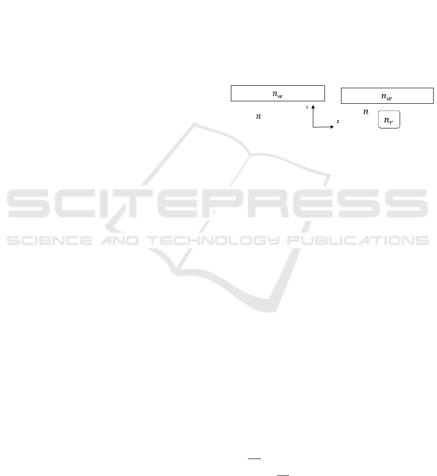
Consider a one-mode resonator side coupled to
waveguide as shown in figure 1. Electromagnetic
fields in the unperturbed waveguide are:
Figure 1: Refractive index distribution of unperturbed
waveguide (right) and perturbed structure (left).
(1)
(2)
Where
and
are transverse mode
profile of the waveguide and
is the operating
angular frequency, and c.c. stands for complex
conjugate of the same term, used for brevity.
Electromagnetic fields in the coupled cavity-
waveguide is approximated as:
(3)
(4)
Where
and
are resonator’s
mode profile and and
are the complex
mode amplitude of the resonator and forward
(backward) mode of the waveguide. Electromagnetic
fields of equations (1) and (2) satisfy Maxwell’s
equation of the unperturbed waveguide, i.e.
and
. Where denotes the permittivity
distribution of the unperturbed structure according to
Figure 1. Similarly, taking the resonator as
PHOTOPTICS 2019 - 7th International Conference on Photonics, Optics and Laser Technology
202

perturbation, a proper expansion of the modes as
given by equation (3) and (4), are the solution of the
equations
and
.
Where is
in the resonator, and zero
elsewhere. Therefore, it’s straightforward to obtain
the following equation:
(5)
By integrating the above equation on the entire x-
y plane and applying time average, high frequency
components become negligible and we can write the
left-hand side of the above equation as:
+
c.c.
]
(6)
Where
represents del operator in transverse
coordinate. According to the two dimensional
divergence theorem one has:
(7)
here the integral is taken on the boundaries of an
infinite circle and represents the vector normal to
the boundaries. As electromagnetic fields decay by
increasing distance from the structure, the above
integral vanishes by integrating in the entire x-y plane.
By assuming orthogonality between mode of the
resonator and waveguide, and assuming that due to
linearity, no frequency conversion occurs, therefore
complex amplitude of the resonator mode is also
single-frequency and in the same frequency with the
waveguide mode. Therefore, equation 5 becomes as
follows:
=
(8)
Where
and electromagnetic fields are
normalized to unit power, i.e.
. The integrals are limited to
resonator boundaries where is non-zero. In the
above equation, integrals represent coupling of the
forward waveguide mode to the resonator, itself and
backward mode, due to the perturbation. Since the
integrals are limited to resonator boundaries, the first
integral is dominant and we have:
(9)
Which is the spatial coupled mode equation for
the “forward mode” in the waveguide and
is
the corresponding coupling coefficient which can be
calculated by the following equation:
(10)
Next the backword mode is considered as the
electromagnetic fields in the unperturbed structure:
(11)
(
(12)
By applying a same procedure, one can obtain the
spatial coupled mode equation for the backward mode
in the waveguide as follows:
(13)
Where the spatial coupling coefficient of the
backward mode to the resonator mode is:
(14)
The mode amplitude in the input ports of the
waveguide is assumed as
and
. Therefore, solving these two equations
with the mentioned boundary conditions, results in:
(15)
Rigorous Derivation of Temporal Coupled Mode Theory Expressions for Travelling and Standing Wave Resonators Coupled to Optical
Waveguides
203
(16)
To obtain transmission and reflection coefficient,
differential equations of the complex mode of the
resonator is needed that is derived in the next section.
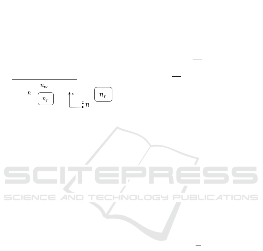
2.1.2 Perturbation of Resonator Mode
In this section the resonator is considered as the
unperturbed structure (figure 2) and effect of adding
a waveguide is studied to derive the differential
equation of the complex mode of the resonator.
Figure 2: Refractive index distribution of unperturbed
resonator (right) and perturbed structure (left).
Therefore, electromagnetic fields in the unperturbed
resonator are:
(17)
(18)
Which due to radiation loss in the optical
resonators, they have limited intrinsic Q-factors. as a
result, modes have complex frequencies. We assume
that resonator is high-Q enough to neglect this effect
for now. In the next section effect of the intrinsic loss
will be considered. By integrating equation (5) on the
entire x-y plane and also from
to
, and using
divergence theorem, we have:
(19)
Since resonator modes decay to zero at infinity,
the last integral which shows integration on the
transverse surfaces in infinity vanishes, and on the
two surfaces in
and
is negligible (by choosing
them far enough from the resonator).
Therefore by substituting electromagnetic fields
of (17),(18) and (3),(4) in equation (5) and applying
time average to omit high frequency components, one
can obtain:
(20)
In the above equation the electromagnetic fields
of the resonator are normalized to have unit energy
i.e.
. According to
figure 2, here
in the waveguide
and is zero elsewhere, is the electric permittivity
distribution of the unperturbed resonator. Hence the
spatial coupled mode equation for forward and
backward modes of the waveguide and a frequency
domain equation for the complex mode amplitude of
the resonator is derived. In the next section, temporal
CMT of the optical coupled cavity-waveguide
structure is obtained with the aid of these equations.
2.1.3 Temporal CMT of Coupled
Cavity-Waveguide
By substituting
and
from (15) and (16)
in (20), temporal CMT for coupled cavity-waveguide
in frequency domain is obtained as follows:
(21)
Where
and
are respectively the self-
induced resonance frequency shift, and the resonance
frequency shift due to coupling to the waveguide.
and
are coupling coefficients of incoming wave of
the ports of the waveguide to the complex mode
amplitude of the resonator and
is the external
decay rate of field amplitude in the resonator. By
applying inverse fourier transform, one can obtain the
time domain equation. The parameters in the above
equation are given as follows:
PHOTOPTICS 2019 - 7th International Conference on Photonics, Optics and Laser Technology
204

.
(22)
(23)
(24)
(25)
Where is given by:
(26)
Transmission and Reflection coefficients are
obtained according to 23 and 24, as follows:
(27)
(28)
2.2 Dual-mode Resonator
In this section the proposed temporal CMT is
generalized to the resonator with two degenerate
modes. A traveling-wave resonator with clockwise
(cw) and counter-clockwise (ccw) modes are
considered for this purpose. This approach is general
and can be applied to any other kind of dual-mode
resonators. The electromagnetic fields in this
structure are expanded as follows:
(29)
(30)
By substituting these fields and the
electromagnetic fields of equation (1) in (2), and
applying the same procedure, one can obtain the
following spatial CMT for the forward mode of the
waveguide:
(31)
By considering electromagnetic fields of the
backward mode in the unperturbed waveguide, spatial
CMT for the backward mode of the waveguide is
obtained as follows:
(32)
Where
(
) and
(
) represent coupling
of the cw to the forward (backward) mode and that of
the ccw to the forward (backward) mode, which are
given as follows:
(33)
(34)
Solving these two equations, results in:
(35)
Rigorous Derivation of Temporal Coupled Mode Theory Expressions for Travelling and Standing Wave Resonators Coupled to Optical
Waveguides
205

(36)
Due to momentum matching, coupling between
forward (backward) and ccw (cw) mode is negligible,
therefore the above equations are simplified as:
(37)
(38)
For obtaining the frequency domain equation for
the complex mode amplitude of the resonator, the
same approach as section 2.1.2 is applied and
resulting equations for the cw and ccw modes are as
follows:
(39)
(40)
Parameters in the above equation are the same as
those in section 2.1.3, except for substituting
with
and
and also
with
and
for parameters in equation (39) and (40)
respectively. A new parameter that shows coupling
between cw and ccw mode is given as follows:
(41)
2.3 Intrinsic Loss
Due to coupling to radiation modes, modes of the
optical resonator undergo intrinsic loss. Thus these
modes are eigenmodes of Maxwell’s equation with
complex frequencies. We enter this effect by
assuming that imaginary part of the complex
frequency represents the internal decay rate of the
field amplitude in the resonator. Therefore,
Electromagnetic fields in the unperturbed resonator
are:
(42)
(43)
Then by assuming that the resonator is high-Q
enough for the mode orthogonality to be
approximately valid, the resulting temporal CMT in
the frequency domain becomes:
(44)
3 RESULTS
In this section, the derived temporal CMT is used to
analyze a square resonator side-coupled to a two port
waveguide, as well as a ring resonator based add drop
filter (four-port structure). FDTD simulations using
Lumerical are used to verify and validate the theory.
3.1 Two-port Structure with Square
Resonator
Consider a square resonator with a standing wave
pattern side coupled to a slab waveguide in the TE
mode as shown in figure 3. The side length of the
resonator, width of the waveguide and edge distance
between resonator and waveguide are ,
PHOTOPTICS 2019 - 7th International Conference on Photonics, Optics and Laser Technology
206
and 0.29 respectively. Refractive index of
the guided regions and background are 3.2 and 1
respectively.
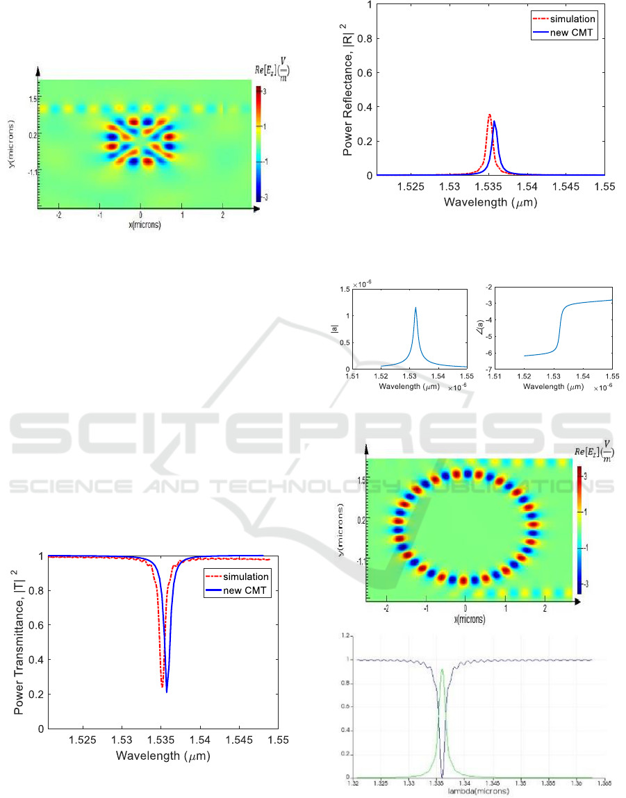
Figure 3: Electric field distribution of the TE mode of the
square resonator near resonance simulated in Lumerical.
Transmission and reflection coefficients of this
structure are calculated with equations derived in
section 2.1.3 and are plotted in figures 4 and 5. The
resonator and waveguide mode in (22) is calculated
via numerical simulations. There is acceptable
agreement between the proposed temporal CMT and
FDTD simulations except for a slight shift between
the resonance frequencies. This error is due to the
approximation of mode orthogonality, or in the other
words, since the resonator has limited intrinsic quality
factor (
), its modes are not orthogonal
anymore. We expect to have better results when
applying the formula to a resonator with higher
quality factor. The amplitude and phase of the
complex mode of the resonator are calculated and
plotted in figure 6.
Figure 4: Power transmission coefficient calculated by the
proposed temporal CMT (solid blue) and FDTD simulation
(dashed red).
Figure 5: Power reflection coefficient calculated by the
proposed temporal CMT (solid blue) and FDTD simulation
(dashed red).
Figure 6: Amplitude (left) and phase (right) of the complex
mode of the resonator.
Figure 7: Electric field distribution of the TE mode of the
ring resonator near resonance (upper) and transmission of
the through (blue) and drop (green) ports simulated in
Lumerical (bottom).
Rigorous Derivation of Temporal Coupled Mode Theory Expressions for Travelling and Standing Wave Resonators Coupled to Optical
Waveguides
207
3.2 Add-drop Filter with Ring
Resonator
An add-drop filter and its TE mode electric field
distribution (calculated with Lumerical) are shown in
figure 7. Radius of the ring, width of the ring and
waveguide, and edge to edge distance between ring
and each waveguide are , and
respectively. Refractive index of the guided regions
and background are 3 and 1 respectively.
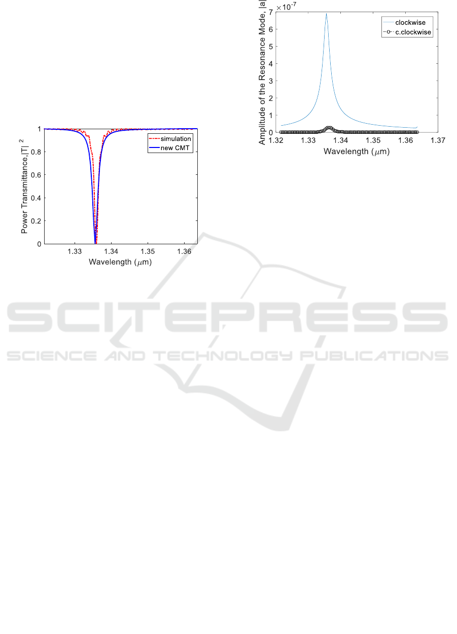
Figure 8: Power transmission coefficient calculated by the
proposed temporal CMT (solid blue) and FDTD simulation
(dashed red).
Since this is a traveling wave resonator that has
two degenerate cw and ccw modes, result of section
2.2 is implemented to calculate transmission and
reflection coefficients and results are plotted in figure
8. In this case, there is better agreement between the
proposed temporal CMT and FDTD simulation,
compared to the previous example. Here the quality
factor of the ring is much higher than the extrinsic
quality factor and effect of intrinsic loss can be
neglected. In the following, amplitude of the complex
cw and ccw modes of the resonator are calculated by
the proposed temporal CMT as shown in figure 9.
Due to the traveling wave nature of the mode, cw
mode is excited mainly and ccw mode amplitude is
negligible.
4 CONCLUSION
In this paper we rigorously derived temporal CMT for
optical cavity-waveguide structures and obtained
closed-form expressions for the coupling coefficients.
Our formulation is general and can be applied to any
kind of resonator, without any prior knowledge. We
demonstrated its validity for structures with standing
wave and traveling wave resonators, and results were
verified against FDTD simulations.
Figure 9: Amplitude of the complex cw (solid blue) and ccw
(line-circle black) mode of the resonator, calculated by the
proposed temporal CMT.
REFERENCES
Agrawal, A., Benson, T., De La Rue, R. and Wurtz, G.
(2017). Recent trends in computational photonics,
Springer Series in Optical Sciences, 1st ed. Cham,
Switzerland :Springer International Publishing.
Fan, S., Suh, W. and Joannopoulos, J. (2003). Temporal
coupled-mode theory for the Fano resonance in optical
resonators. Journal of the Optical Society of America A,
20(3), p.569.
Haus, H. (1984). Waves and fields in optoelectronics.
Marietta, Ohio: CBLS.
Haus, H. and Huang, W. (1991). Coupled-mode
theory. Proceedings of the IEEE, 79(10), pp.1505-1518.
Kristensen, P., de Lasson, J., Heuck, M., Gregersen, N. and
Mork, J. (2017). On the Theory of Coupled Modes in
Optical Cavity-Waveguide Structures. Journal of
Lightwave Technology, 35(19), pp.4247-4259.
Little, B., Chu, S., Haus, H., Foresi, J. and Laine, J. (1997).
Microring resonator channel dropping filters. Journal
of Lightwave Technology, 15(6), pp.998-1005.
Li, Q., Wang, T., Su, Y., Yan, M. and Qiu, M. (2010).
Coupled mode theory analysis of mode-splitting in
coupled cavity system. Optics Express, 18(8), p.8367.
Manolatou, C., Khan, M., Fan, S., Villeneuve, P., Haus, H.
and Joannopoulos, J. (1999). Coupling of modes
analysis of resonant channel add-drop filters. IEEE
Journal of Quantum Electronics, 35(9), pp.1322-1331.
Pierce, J.R., (1954). Coupling of Modes of
Propagation. Journal of Applied Physics, 25(2), pp.179–
183.
Wonjoo Suh, Zheng Wang and Shanhui Fan (2004).
Temporal coupled-mode theory and the presence of
non-orthogonal modes in lossless multimode
cavities. IEEE Journal of Quantum Electronics, 40(10),
pp.1511-1518.
Yariv, A. (1973). Coupled-mode theory for guided-wave
optics. IEEE Journal of Quantum Electronics, 9(9),
pp.919-933.
PHOTOPTICS 2019 - 7th International Conference on Photonics, Optics and Laser Technology
208
