More Accurate Pose Initialization with Redundant Measurements
Ksenia Klionovska, Heike Benninghoff and Felix Huber
German Aerospace Center, Muenchener street, 20, Wessling, Germany
Keywords:
Photonic Mixer Device (PMD) Sensor, 3D-2D Pose Estimation, Hough Line Transform.
Abstract:
The problem described in this paper concerns the problem of initial pose estimation of a non-cooperative
target for space applications. We propose to use a Photonic Mixer Device (PMD) sensor in a close range
for the visual navigation in order to estimate position and attitude of the space object. The advantage of the
ranging PMD sensor is that it provides two different sources of data: depth and amplitude information of the
imaging scene. In this work we make use of it and propose a follow-up initial pose improvement technique
with the amplitude images from PMD sensor. It means that we primary calculate the pose of the target with
the depth image and then correct the pose to get more accurate result. The algorithm is tested for the set of
images in the range 8 to 4.9 meters. The obtained results have shown the evident improvement of the initial
pose after correction with the proposed technique.
1 INTRODUCTION
Computer vision is a huge branch, which allows com-
puters to understand and process images for different
applications, e.g. autonomous driving, health care,
agriculture, industrial. Our research is aimed to use
computer vision for the aerospace applications. The
goal is to estimate an initial pose (position and atti-
tude) of the unknown space object without any previ-
ous knowledge about it.
The state-of-the-art techniques for pose initiali-
zation in space are presented in follow works. In
the article of (Sharma et al., 2018) authors pro-
pose the model based initial pose estimation of the
non-cooperative spacecraft with monocular vision.
The other approach (Rems et al., 2015) suggests to
use LIDAR’s 3D point clouds for acquisition of the
unknown pose of the space object. In the follow paper
(Klionovska and Benninghoff, 2017) authors show
an approach for pose acquisition with the 3D data
obtained from a time-of-flight Photonic Mixer Device
(PMD) sensor, which can be considered as possible
candidate for visual navigation in future space missi-
ons. PMD sensor provides the raster depth image of
the imaging scene, which is calculated using the phase
shift delay between emitted and reflected signals.
Since we continue investigating further possibility
of PMD sensor, especially its robustness to estimate a
pose of the space object, in this work we introduce a
follow-up improvement technique for initial pose re-
finement. It should be mentioned that the depth PMD
sensor provides not only depth image, but also has
an ability to generate co-registered amplitude data. It
means: at the beginning we calculate the initial pose
of the non-cooperative vehicle with the depth image,
namely, with the correspondent point cloud, and after
that, the obtained pose is corrected with a correspon-
dent method using the amplitude image. The algo-
rithm which is proposed to apply for the amplitude
image consists of the image processing technique in
order to detect the straight lines and end points of the
lines, and successive Gauss-Newton minimization for
the pose determination.
For verification of the algorithms with the PMD
sensor at German Aerospace Center we run simulati-
ons with the high accuracy hardware-in-the-loop Eu-
ropean Proximity Operations Simulator (EPOS 2.0)
(Benninghoff et al., 2017) and with a prototype DLR-
Argos3D - P320 camera provided by Bluetechnix
company. We do tests and evaluate the results for the
initial pose estimation in the close range 8 to 4.9 me-
ters.
2 PROBLEM STATEMENT
The problem of the initial pose estimation of the non-
cooperative target can be described as follows. We
assume to have on board a 3D model of the target, see
Figure 1, presented in a body frame. The optical pro-
146
Klionovska, K., Benninghoff, H. and Huber, F.
More Accurate Pose Initialization with Redundant Measurements.
DOI: 10.5220/0007378001460153
In Proceedings of the 14th International Joint Conference on Computer Vision, Imaging and Computer Graphics Theory and Applications (VISIGRAPP 2019), pages 146-153
ISBN: 978-989-758-354-4
Copyright
c
 2019 by SCITEPRESS – Science and Technology Publications, Lda. All rights reserved

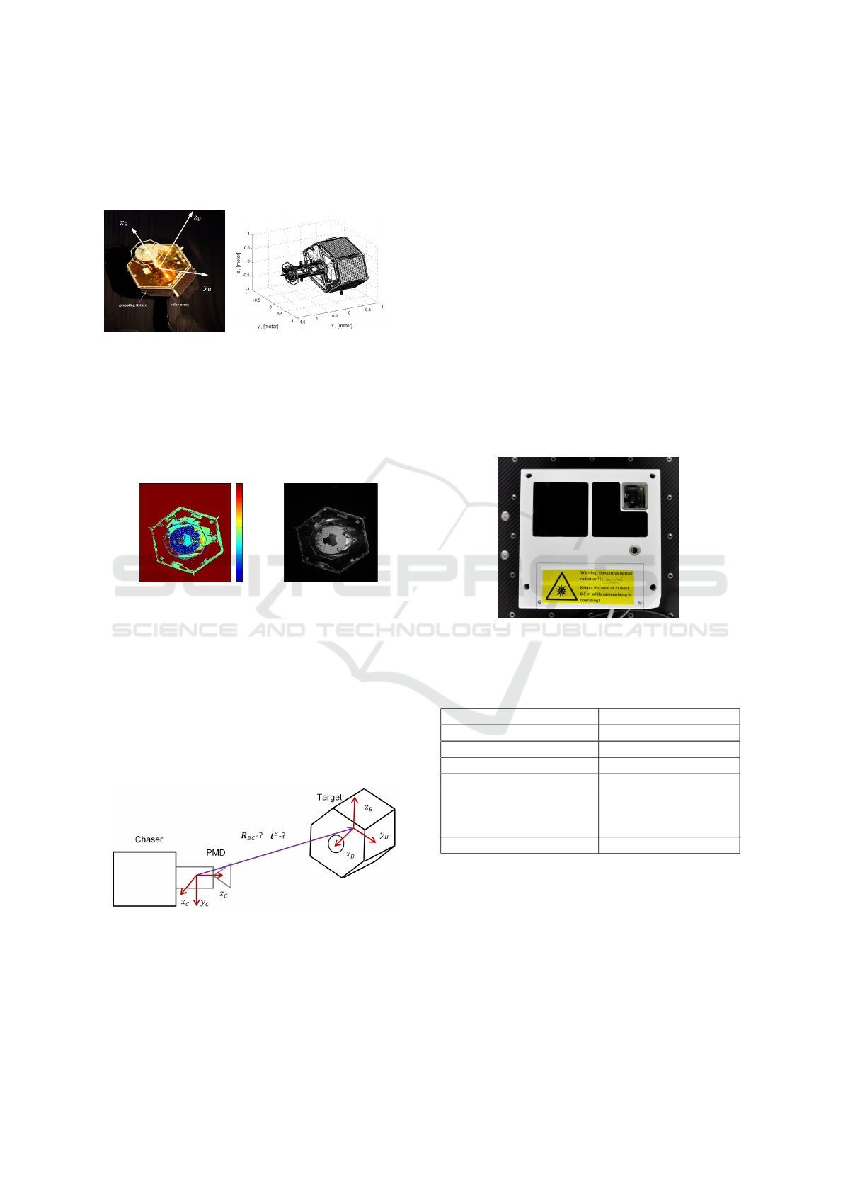
perties of the mockup’s surface materials are similar
with the real ones used in space. In the future we are
planning to test the proposed techniques with PMD
sensor using different 3D targets.
Figure 1: Image of Target in EPOS Laboratory and Its 3D
Model.
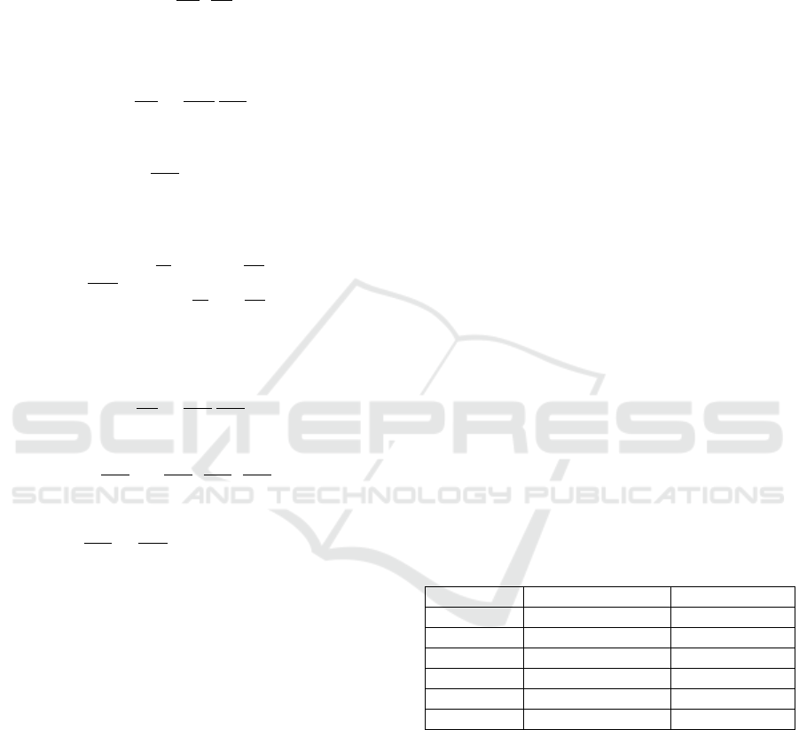
The PMD sensor attached to the chaser provides
co-registered depth and amplitude images of the tar-
get. The example of these images is depicted in Fi-
gure 2. We would like to note that amplitude image
can be treated as a 2D gray-scaled image. Therefore,
pixel
pixel
50 100 150 200 250
50
100
150
200
250
300
350
millimeters
0
1000
2000
3000
4000
5000
6000
7000
8000
9000
pixel
pixel
50 100 150 200 250
50
100
150
200
250
300
350
Figure 2: Depth and Amplitude Images taken with DLR-
Argos 3D-P320 Camera .
the task is to determine accurately the relative posi-
tion vector t
b
and relative attitude of the target using
only these two sources of information: 3D known mo-
del and obtained PMD image. The relative attitude
defines the rotation matrix R
bc
from body coordinate
frame to the camera frame. The sketch of the coordi-
nate systems, as well as unknown position and orien-
tation are presented in Figure 3.
Figure 3: Coordinate Systems of the Attached PMD Sensor
and Target.
3 METHODS
In the previous section we have determined the pro-
blem of the initial pose estimation. Since we are tes-
ting the PMD sensor for this purpose, we are going to
present the sensor and its features. Further the des-
cription of the follow-up pose correction technique
using an amplitude image of PMD sensor is provided.
3.1 DLR-Argos 3D-P320 Camera
The depth measurement principle of the PMD techno-
logies is based on the calculation of the phase shift
between the emitted NIR signal by the LED’s of the
camera and reflected signal from the target. The am-
plitude data shows the strength of the reflected signal
from the object. The characteristics of the PMD sen-
sor used in this paper are presented in Table 1 and the
image of the camera is plotted in Figure 4.
Figure 4: DLR-Argos 3D-P320 Camera in EPOS Labora-
tory.
Table 1: Technical Characteristics of the PMD Sensor In-
side the DLR-Argos 3D-P320 Camera.
Field of View (FOV) 28.91 x 23.45 deg
Resolution of the chip 352 x 287 pixels
Integration time 24 ms
Frames per second 45
Modulated frequencies 5.004 MHz, 7.5 MHz,
10.007 MHz, 15 MHz,
20.013MHz,
25.016 MHz, 30MHz
Mass/Power consumption 2 kg/ < 25.5W
We should underline that using proposed mockup
with its surfaces we are able to initialize pose only
from the front side. This is because of the inability of
the PMD camera to provide correct depth measure-
ments when one is working with high absorbing sur-
faces, e.g solar arrays. In Figure 1 (left image), we
denote solar arrays of the used mockup in the EPOS
laboratory.
More Accurate Pose Initialization with Redundant Measurements
147

3.2 Follow-up Refinement of Initial Pose
with Amplitude Image
In the paper of Klionovska et al. (Klionovska and
Benninghoff, 2017), we propose the algorithm which
we used in order to acquire the pose of the non-
cooperative target using the depth image of PMD sen-
sor and known 3D model. In that paper, we have dis-
covered differednet things: the use of a proper shape
(a frontal hexagon and a ”nose”) of the 3D model is
a prerequisite for the correct work of the algorithm;
the determination of the attitude of the target using
only point cloud from the depth image is a deman-
ding problem. Specifically, the determination of the
target’s rotation around its principal axis of inertia (in
Figure 1 (left) is an axis x
B
) only with the 3D point
cloud depth data can lead to misalignments up to 30
degrees. The other rotational components can also be
affected. Since it is preferable to have an accurate
initial guess for the tracker in order to navigate to the
target in a frame-to-frame mode, we propose an initial
pose refinement with the amplitude image.
In the work of Klionovska et al. (Klionovska et al.,
2018) we presented for the first time a navigation sy-
stem which uses depth and amplitude images from the
PMD sensor. We have shown that the use of ampli-
tude image along with the depth image for the pose
estimation leads to stable tracking, since the ampli-
tude information can be considered as a redundant
and let us calculate a pose when the depth algorithm
fails or gives wrong measurements. Moreover, it was
shown that (partly) lost distance information of the
target from the depth images is still present in the
amplitude images. It means that with the amplitude
image we can get a more complete representation of
the imaging target, consequently, more accurate esti-
mation of the pose. And finally, the model-base pose
estimation technique with the 2D amplitude image de-
monstrates more accurate estimation of the attitude of
the target in comparison with the 3D pose estimation
technique.
Having analyzed the pros of using the amplitude
image for the pose estimation during the tracking, we
have decided to apply it as a supplement processing
for the enhancement of the initial pose. We assume
to have the essential estimated pose of the target af-
ter pose initialization technique with the depth image.
It means that the proposed technique with the ampli-
tude image has already kind of a guess pose as an
input, which is a necessary prerequisite for the cho-
sen improvement technique. For the initial pose re-
finement, we are going to apply an image processing
technique based on the line detection procedure with
Hough Line Transform. The detected straight lines,
namely the end points of that lines, will be the feature
points in order to get the pose by solving 3D-2D pro-
blem. Throughout variety of the solvers (Sharma and
D’Amico, 2016), here we propose to take a Gauss-
Newton solver based on a least square minimization
problem (Nocedal and Wright, 2006) (Cropp, 2001)
in order to estimate the pose of the target related to
the camera frame. The Gauss-Newton solver iterati-
vely solves perspective projection equations with the
known first guess. Let us consider the image proces-
sing technique and Gauss-Newton solver.
3.2.1 Image Processing
Since we are able to estimate the initial pose only
from the front side of the mockup, the visible front
hexagon is defined as an appropriate feature. The hex-
agon is constructed with six straight lines, which are
completely observable if the target is in the FOV of
the camera. The image processing pipeline in order
to detect straight lines has follow steps (HoughLine-
Transform, 2009):
• Use of low-pass filtering to reduce image noise
• Execution of Canny-edge operator (Canny, 1986)
for the edge extraction in the amplitude images
• Employment of Probabalistic Hough Line Trans-
form for finite lines detection
The straight lines give us also the end points,
which are assumed to be the detected features. Kno-
wing the initial pose defined by the depth image, cal-
led guess pose T
guess
, and calibration matrix A of the
PMD sensor, the 3D model can be re-projected onto
the image plane, see Figure 5 (left). The calibration
matrix A is presented by
A =


α γ u
0
0 β v
0
0 0 1


(1)
and includes the following parameters: focal lengths
α and β, coordinates of the principal point (u
0
,v
0
) and
a skew factor γ between x and y axis. We determi-
ned the calibration matrix of the current PMD sensor
in the paper of Klionovska et al. (Klionovska et al.,
2017) using DLR CalDe and DLR CalLab Calibration
Toolbox. After 3D model re-projection, there are two
sets of points in the image: detected feature points
from the image and re-projected points of the 3D mo-
del. By finding nearest neighbors between them a list
of feature correspondences, as in Figure 5 (right), can
be generated.
3.2.2 Gauss-Newton Solver
The following step is to calculate the pose of the spa-
cecraft with respect to the known 3D-2D feature cor-
VISAPP 2019 - 14th International Conference on Computer Vision Theory and Applications
148

Figure 5: Left: Re-projection of the 3D Model with Pose Estimated by Depth Image. Right: Neighbors Found for Re-projected
3D Model and Detected End Points of the Image.
respondences. We assume that during image proces-
sing with the Hough Line Technique we obtained a
set of image points r
img
= [u,v]
T
and a set of corre-
sponding model points p
T
=

p
x
T
, p
y
T
, p
z
T

T
.
Let us consider the pose (R
C
T
,t
C
) as a 6 parameters
vector x = [t
C
T
,θ], where t
C
T
is position vector with
respect to the camera frame, and θ = [θ
1
,θ
2
,θ
3
] is set
of the Euler angles, which determines the orientation
of the target spacecraft. The projection of the point
p
T
on the image is obtained through the 3D-2D true
perspective projection equations:
p
C
= R
C
T
p
T
+t
C
(2)
ρ
M
=

u
v

=


p
x
C
p
z
C
α + u
0
p
y
C
p
z
C
β + v
0


(3)
In Equation 2 and Equation 3 p
T
is the feature point
of the target model defined in the target frame, p
C
is
the same point in a camera frame after applying trans-
formation (R
C
T
,t
C
) , (u,v) is the pixel of the image
corresponding to the feature, (α,β) focal lengths of
the camera and (u
0
,v
0
) principal point of the camera.
Equation 3 uses simple camera model, where only fo-
cal lengths and principal point of the camera are taken
from Equation 1. For each coupled feature correspon-
dence image-model it is possible to define the follo-
wing residual error:
e = ρ
M
− ρ
img
=

u
M
(x) − u
img
v
M
(x) − v
img

(4)
where ρ
M
is the projection of the geometric feature
of the target model, whereas ρ
img
is the end point de-
tected with the Hough Line Transform. The error in
the Equation 4 has six unknown parameters, which
are described by the state vector x. The state vector
contains three Euler angle, which define the rotation
matrix and three coordinates of the translation vec-
tor. Each feature correspondence is defined by two
conditions, therefore, at least three pairs of matches
between detected end points and projected features
are required to solve the system equation for the de-
fined error function. Let us assume that we have N
feature correspondences between image and model
points. The Gauss-Newton approach iteratively mi-
nimizes the sum of square errors in order to find the
position and orientation defined by x.
S(x) =
N
∑
i=1
ke
i
(x)k
2
=
N
∑
i=1
[(u
i
(x)−u
i
)
2
+(v
i
(x)−v
i
)
2
].
(5)
Given the first guess x
0
, the pose that minimizes
Equation 5 is iteratively obtained as
x
k+1
= x
k
− (J
T
k
J
k
)
−1
J
T
k
E
k
(6)
where
E
k
=



e
1
(x
k
)
e
2
(x
k
)
..
e
N
(x
k
)



(7)
is the error vector with e
i
defined in the Equation 4
and J
k
is the Jacobian of e calculated at x
k
and defined
as
J =
∂e
∂x
. (8)
The equation for the Jacobian (8) for point corre-
spondences can be written as follow:
J =

∂e
∂t
C
,
∂e
∂θ

=



∂e
1
∂t
C
∂e
1
∂θ
....
∂e
N
∂t
C
∂e
N
∂θ



. (9)
More Accurate Pose Initialization with Redundant Measurements
149

The size of the Jacobian is 2Nx6 since each resi-
dual error in the Equation 4 is defined by two compo-
nents along u and v coordinates of the image.
The general expression of the rows of the Jacobian
being
J
i
=

∂e
i
∂t
C
,
∂e
i
∂θ

. (10)
In the Equation 10, e
i
= ρ
M
− ρ
img
, i = 1...N.
The first element of the row can be rewritten as
∂e
i
∂t
C
=
∂ρ
M
∂p
C
∂p
C
∂t
C
(11)
where
∂p
C
∂t
C
= I
3×3
(12)
and the follow equation obtained from Equation 2 and
Equation 3
∂ρ
M
∂p
C
=


α
p
C
z
0 −
p
C
x
p
C2
z
α
0
β
p
C
z
−
p
C
y
p
C2
z
β


. (13)
Alternatively, the second element of the Equation 10
can be presented as
∂e
i
∂θ
=
∂r
M
∂p
C
∂p
C
∂θ
(14)
with
∂p
C
∂θ
=

∂p
C
∂θ
1
,
∂p
C
∂θ
2
,
∂p
C
∂θ
3

(15)
and
∂p
C
∂θ
j
=
∂R
C
T
∂θ
j
p
T
j = 1, 2, 3. (16)
In the Equation 16, the rotation matrix defined in
terms of Euler angles [θ
1
,θ
2
,θ
3
] as
R
C
t
=


cθ
1
cθ
1
sθ
1
sθ
1
−sθ
2
cθ
1
sθ
2
sθ
3
− sθ
1
cθ
3
sθ
1
sθ
2
sθ
3
+ cθ
1
cθ
3
cθ
2
sθ
3
cθ
1
sθ
2
sθ
3
+ sθ
1
sθ
3
sθ
1
sθ
2
sθ
3
− cθ
1
sθ
3
cθ
2
cθ
3


(17)
where cθ = cosθ and sθ = sin θ.
4 RESULTS
The DLR-Argos3D - P320 sensor is able to work pro-
perly with the given mockup and chosen scenario in
the range from 8 to 4.9 m. The maximum working
range 8 meters is chosen because of the camera’s LED
power and resolution of the sensor chip. The mini-
mum working distance is defined in dependence on
the camera FOV. If the distance is less than 4.9 m, the
whole contour of hexagon cannot be observed in some
parts. We are going to test proposed follow-up refine-
ment of the initial pose for two data sets. The first
data set contains 163 images in the distance range 8
to 7 m from the target. The second data set contains
30 images in the distance range 7 to 4.9 m. The bigger
amount of images for the first data set is taken purpo-
sely, because we are interested to test initial pose es-
timation with the given PMD sensor in the far range
region. As soon as we estimate the initial pose, we
can start to approach the target in a frame-to-frame
mode. The tracking is out of scope in this paper.
Some remarks to the evaluation of the initial pose.
According to the target symmetry along its principal
axis, the errors in the roll angle always lie in the range
from 0 to 30 deg. Moreover, even if the errors in a roll
angle are small, it can happen that the re-projection
of the model’s octagon onto the image doesn’t match
it. It means that there is a need to use any additional
technique, which takes into account octagon shape for
its correct determination. The numerical errors in the
following sections are obtained by comparing the al-
gorithms output and ground truth from the EPOS.
4.1 Distance Range 8 to 7 Meters
We execute the pose initialization technique with the
depth images and thereafter run the follow-up initial
pose refinement with the amplitude images for the
first data set. In Table 2 the mean errors in the cal-
culated initial pose with and without correction are
presented. The ground truth from the EPOS facility
was use for calculation of the errors.
Table 2: Mean Error of the Initial Estimated Pose with and
without Correction for the First Data Set.
mean value without correction with correction
µ
roll
, deg 13.387 0.788
µ
pitch
,deg 1,960 0.492
µ
yaw
, deg 1,594 0.525
µ
z
, m 0.1293 0.0805
µ
y
,m 0.0436 0.0201
µ
x
,m 0.0226 0.0108
From the Table 2 one can observe more accurate
estimation of the attitude and position of the initial
pose after application of the initial pose refinement
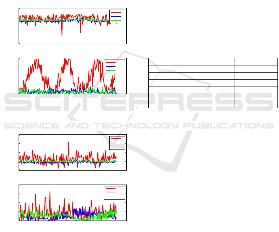
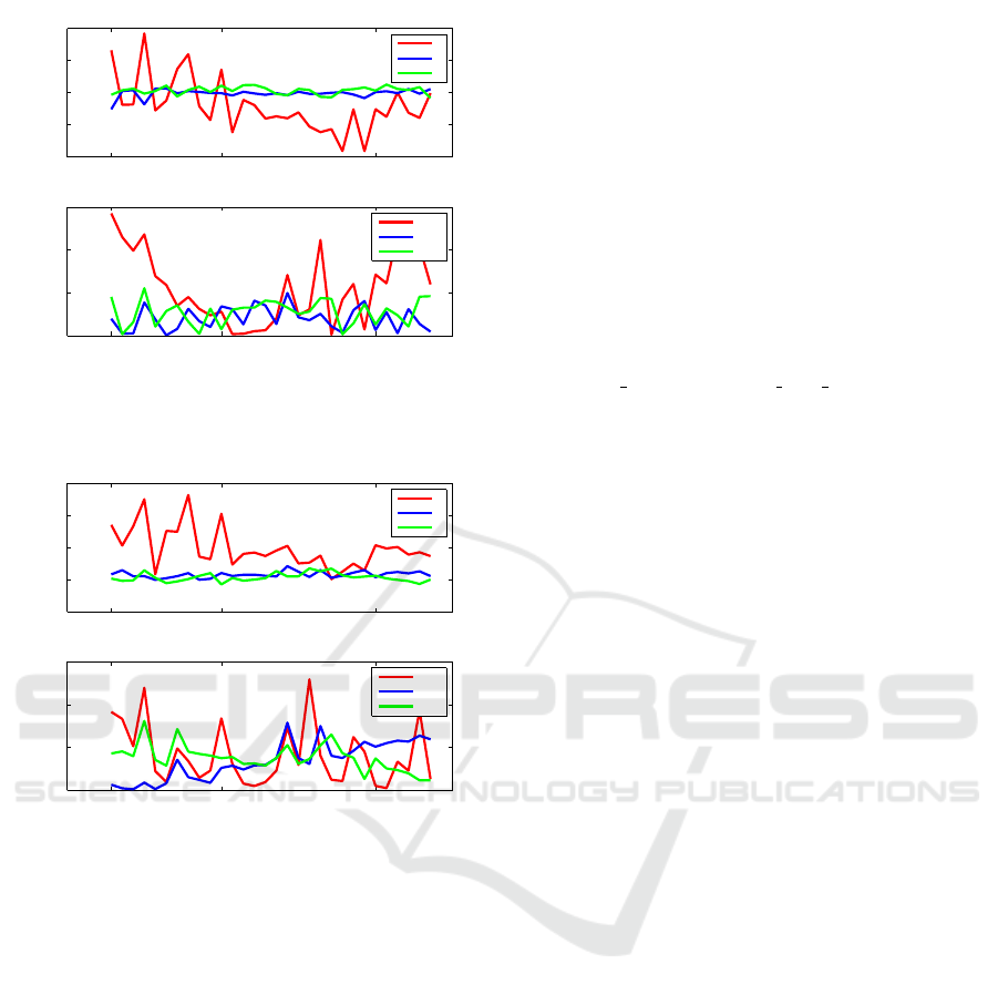
with amplitude image. In Figure 6 (down) it can be
noticed that in many cases we cannot properly define
the initial rotation of the target around it’s principle
axis using only depth information. Nevertheless, this
never happens after initial pose refinement, see Figure
7 (down). The mean value for the roll angle µ
roll
of
the essential initial pose reaches 13.387 deg and the
maximum 29.87 deg, whereas the µ
roll
value for the
corrected pose is 0.788 deg and the maximum value
VISAPP 2019 - 14th International Conference on Computer Vision Theory and Applications
150

reached 3.207 deg. Concerning the estimation of the
initial position in the range from 8 to 7 m, one can
observe that the mean error µ
z
for the distance measu-
rements between target and chaser without correction
is 0.1293 m, and for the corrected pose it is 0.0805
meters. For the position errors along two other axis y
and x the mean errors µ
y
and µ
x
are two times less than
for the corrected initial pose, see Table 2. In Figure
A2 we present some amplitude images in the range
from 8 to 7 m with the resulted poses of the target.
Every row contains two pairs of poses: calculated ini-
tial pose without correction and refined pose with the
amplitude.
8 7
−1
−0.5
0
0.5
distance to the target, meters
error, meters
z
y
x
8 7
0
10
20
30
distance to the target, meters
error, deg
roll
pitch
yaw
Figure 6: Translation and Rotation errors for the initial es-
timated pose only with the depth data in the range from 8 to
7 meters.
8 7
−0.2
0
0.2
0.4
0.6
distance to the target, meters
error, meters
z
y
x
8 7
0
1
2
3
4
distance to the target, meters
error, deg
roll
pitch
yaw
Figure 7: Translation and Rotation errors for the corrected
initial estimated pose in the range from 8 to 7 meters.
4.2 Distance Range 7 to 4.9 Meters
Let us consider the results of the initial pose estima-
tion of the second data set with and without correecti-
ons in the range from 7 to 4.9 m. It should be noticed
that the closer the camera to the target, the bigger the
size of the point cloud. In our previous paper (Klio-
novska and Benninghoff, 2017), where we discussed
the pose initial algorithm with the depth data, it was
mentioned the fact that the depth algorithm is sensi-
tive to the size of the point cloud. If the point cloud
of a scene has a big amount of points, it can happen
that the accuracy of the initial pose drops. This is due
to the fact that the close to the target, more details can
be observed and measured by the camera. The scene
point cloud will be more dense than the model, and
this could lead to some misalignment. Actually, we
can see this in Figure 8 (down), where the errors in de-
termining yaw and pitch angles for the second data set
are evidently higher than in the first data set in Figure
6 (down). From the Table 3, where the mean errors
are summed up for the position and orientation of the
estimated initial poses, one can notice the significant
advantages of the follow-up initial pose correction.
Table 3: Mean Error of the Initial Estimated Pose with and
without Correction for the Second Data Set.
mean value without correction with correction
µ
roll
,deg 11.304 0.821
µ
pitch
,deg 3.989 0.682
µ
yaw
,deg 5.450 0.760
µ
z
,m 0.1581 0.0972
µ
y
,m 0.0157 0.0157
µ
x
,m 0.0224 0.0109
Let us consider one case in more details. In Fi-
gure A2, we again print some pairs of amplitude ima-
ges and the resulted pose calculated with and without
correction for the second data set. Two images from
the left of the last row in Figure A2 reflect initial pose
at the distance 4.9 m. The attitude errors of the uncor-
rected initial pose occur for the roll, pitch and yaw
angles are 23.562 deg, 0.5333 deg and 4.734 deg.
The position errors along x, y and z axis are 0.0231
m, 0.0034 m, 0.0006 m. The errors for the corrected
pose: roll - 0.669 deg, pitch - 1.160 deg and yaw -
0.471 deg; position along x, y and z axis are 0.0009
m, 0.0236 m, 0.1016 m. Having a look at Figure
8 and Figure 9 one can notice that this was exactly
an unique case, when the depth coordinate without
correction was calculated extremely accurate in com-
parison with the corrected result. Nevertheless, the
mean value µ
z
=0.0109 m for the corrected initial pose
is much better than the µ
z
=0.0224 m for the primary
estimated pose.
5 CONCLUSION
In this paper, we presented the improvement techni-
que for the initial pose estimation of the non-
More Accurate Pose Initialization with Redundant Measurements
151

7 6 5
−0.4
−0.2
0
0.2
0.4
distance to the target, meters
error, meters
z
y
x
7 6 5
0
10
20
30
distance to the target, meters
error, deg
roll
pitch
yaw
Figure 8: Translation and Attitude Errors for the Initial Es-
timated Pose only with Depth Data in the Range from 7 to
4.9 Meters.
7 6 5
−0.1
0
0.1
0.2
0.3
distance to the target, meters
error, meters
z
y
x
7 6 5
0
1
2
3
distance to the target, meters
error, deg
roll
pitch
yaw
Figure 9: Translation and Attitude Errors for the Corrected
Initial Estimated Pose in the Range from 7 to 4.9 Meters.
cooperative target for space missions with relatively
new time-of-flight PMD sensor. The proposed appro-
ach takes into account the additional amplitude data
of the PMD sensor provided in parallel to the depth
measurements. This feature leads to the software re-
dundancy without hardware redundancy. As soon as
a primary initial pose can be calculated with the depth
image, the following pose refinement technique takes
place for more accurate acquisition of the position and
orientation of the unknown target using a single PMD
sensor. Conducting experiments with the real ima-
ges of PMD sensor and the existent mockup, we have
shown the necessity of the follow-up initial pose re-
finement, since it crucially increases the accuracy of
the estimated pose.
REFERENCES
Benninghoff, H., Rems, F., and Risse, E. (2017). Eu-
ropean proximity operations simulator 2.0 (EPOS) -
a robotic-based rendezvous and docking simulator.
Journal of large-scale research facilities, 3.
Canny, J. (1986). A computational approach to edge de-
tection. IEEE Transactions on Pattern Analysis and
Machine Intelligence, (6).
Cropp, A. (2001). Pose estimation and relative orbit deter-
mination of a nearby target microsatellite using pas-
sive imagery. PhD Thesis, University of Surrey.
HoughLineTransform (2009). Hough
Line Transform. Available at htt p :
//web.ipac.caltech.edu/sta f f / f masci/home/
/astro re f s/HoughTrans lines 09.pd f .
Klionovska, K. and Benninghoff, H. (2017). Initial pose
estimation using PMD sensor during the rendezvous
phase in on-orbit servicing missions. 27th AAS/AIAA
Space Flight Mechanics Meeting, Texas, USA.
Klionovska, K., Benninghoff, H., and Strobl, K. H.
(2017). PMD Camera-and Hand-Eye-Calibration for
On-Orbit Servicing Test Scenarios On the Ground.
14th Symposium on Advanced Space Technologies in
Robotis and Automation (ASTRA),Leiden, the Nether-
lands.
Klionovska, K., Ventura, J., Benninghoff, H., and Huber,
F. (2018). Close range tracking of an uncooperative
target in a sequence of photonic mixer device (pmd)
images. Robotics, 7.
Nocedal, J. and Wright, S. (2006). Numerical optimization.
Springer-Verlag New York.
Rems, F., Moreno Gonzalez, J. A., Boge, T., Tuttas, S., and
Stilla, U. (2015). Fats initial pose estimation of spa-
cecraft from lidar point cloud data. 13th Symposium
on Advanced Space Technologies in Robotics and Au-
tomation.
Sharma, S. and D’Amico, S. (2016). Comparative asses-
sment of techniques for initial pose estimation using
monocular vision. Acta Astronautica, 123.
Sharma, S., Ventura, J., and D’Amico, S. (2018). Robust
model-based monocular pose initialization for non-
cooperative spacecraft rendezvous. Journal of Spa-
cecraft and Rockets, pages 1–16.
APPENDIX
Assumptions: Column I is a initial pose without cor-
rection. Column II is a initial pose corrected with the
proposed technique.
VISAPP 2019 - 14th International Conference on Computer Vision Theory and Applications
152

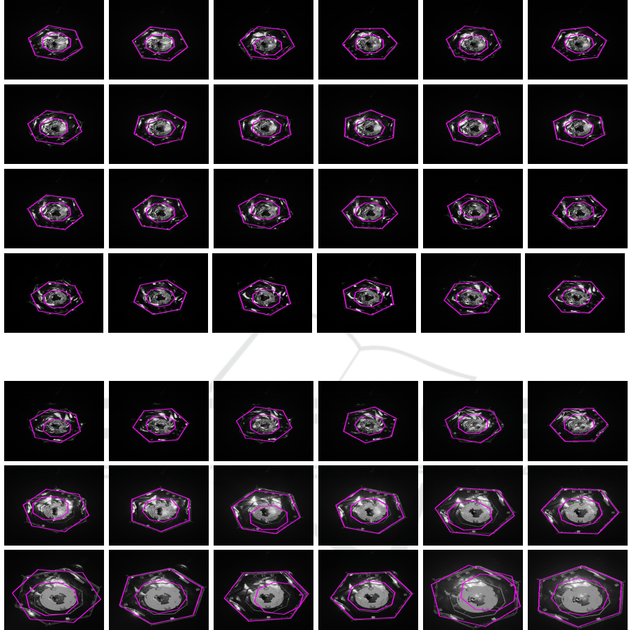
I II I II I II
Figure A1: Set of Some Amplitude Images in Range 8 to 7 Meters with Uncorrected and Corrected Initial Poses.
I II I II I II
Figure A2: Set of Some Amplitude Images in Range 7 to 4.9 Meters with Uncorrected and Corrected Initial Poses.
More Accurate Pose Initialization with Redundant Measurements
153