Exploring the Limitations of the Convolutional Neural Networks on
Binary Tests Selection for Local Features
Bernardo Janko Gonc¸alves Biesseck
1,2
, Edson Roteia Araujo Junior
1
and Erickson R. Nascimento
1
1
Universidade Federal de Minas Gerais (UFMG), Brazil
2
Instituto Federal de Mato Grosso (IFMT), Brazil
Keywords:
Binary Tests, Keypoint Descriptor, Convolutional Neural Network.
Abstract:
Convolutional Neural Networks (CNN) have been successfully used to recognize and extract visual patterns
in different tasks such as object detection, object classification, scene recognition, and image retrieval. The
CNNs have also contributed in local features extraction by learning local representations. A representative
approach is LIFT that generates keypoint descriptors more discriminative than handcrafted algorithms like
SIFT, BRIEF, and SURF. In this paper, we investigate the binary tests selection problem, and we present an
in-depth study of the limit of searching solutions with CNNs when the gradient is computed from the local
neighborhood of the selected pixels. We performed several experiments with a Siamese Network trained with
corresponding and non-corresponding patch pairs. Our results show the presence of Local Minima and also a
problem that we called Incorrect Gradient Components. We pursued to understand the binary tests selection
problem and even some limitations of Convolutional Neural Networks to avoid searching for solutions in
unviable directions.
1 INTRODUCTION
Local floating point descriptors, such as SIFT (Lowe,
2004), SURF (Bay et al., 2006), and HOG (Dalal and
Triggs, 2005), are well known in literature as being
discriminative and robust to rotation, scale, and illu-
mination changes in images. However, they have a
high computational cost and are expensive to store,
which make difficult running these float descriptors
on computers with limited hardware (e.g., embedded
systems, smartphones, etc.) when the number of ima-
ges and descriptors are large.
A popular approach to reduce computational cost
is to design a local feature extractor that creates binary
descriptors. Designed to be fast, binary descriptors
are based on binary tests that compare pixels inten-
sities around a keypoint. While each SIFT descriptor
occupies 512 bytes of memory and uses the Euclidean
distance as a similarity measure, a BRIEF (Calonder
et al., 2010) descriptor, for instance, needs 32 Bytes
and uses Hamming distance to compare two feature
vectors.
The past decade has witnessed an explosion of
similar approaches to BRIEF, each one using a dif-
ferent binary tests set. ORB (Rublee et al., 2011),
BRISK (Leutenegger et al., 2011) and FREAK (Or-
tiz, 2012) are three descriptors that explore different
image properties and spatial pattern of binary tests to
improve their robustness and matching performance.
Recently, binary descriptors based on Convolutional
Neural Networks (CNN) have been created, such as
DeepBit (Lin et al., 2016) and DBD-MQ (Duan et al.,
2017). However, these CNN-based methods still have
high computational cost because of the several layers
of the deep networks used on their solutions.
Virtually all binary descriptors define a spatial pat-
tern to be used to select the pixels when extracting the
local features. Beyond being a common step on bi-
nary descriptors, the spatial pattern is crucial for the
matching performance. Motivated to discovering new
patterns of binary tests, we propose to answer the fol-
lowing question: Is a CNN-based model able to find a
spatial distribution of binary test that minimizes dis-
tances between corresponding keypoints and maximi-
zes distances between non-corresponding keypoints?
Our idea is to use the CNN power to extract distri-
butions not yet observed by the scientific community.
Our results demonstrate two significant hindrances to
the use of CNN on binary tests selections: the ex-
istence of Local Minima and what we called Incor-
rect Gradient Components. These two problems ap-
pear when the objective function gradient (used in the
Biesseck, B., Araujo Junior, E. and Nascimento, E.
Exploring the Limitations of the Convolutional Neural Networks on Binary Tests Selection for Local Features.
DOI: 10.5220/0007374102610271
In Proceedings of the 14th International Joint Conference on Computer Vision, Imaging and Computer Graphics Theor y and Applications (VISIGRAPP 2019), pages 261-271
ISBN: 978-989-758-354-4
Copyright
c
 2019 by SCITEPRESS – Science and Technology Publications, Lda. All rights reserved
261

Back-propagation step) is calculated from the local
pixel’s neighborhood. As main contribution, we pre-
sent in this paper some limitations of CNN in binary
tests selection to understand the robustness and the li-
mits of using CNNs on binary tests selection for local
feature extraction.
2 RELATED WORK
Binary descriptors have been presented as alternative
approaches to floating point descriptors. They are
useful mainly in applications running on computers
with limited resources, such as embedded systems,
smartphones, etc. A binary descriptor is composed
of bits that are, in general, the result of binary tests
defined as
τ(I, x, y, w, z) =
(
1 if I(x, y) < I(w, z),
0 otherwise,
(1)
where I(x, y) and I(w, z) are the intensities of pixels
(x, y) and (w, z) of a digital image I. Each binary test
compares two pixels and a set of n binary tests com-
pose a binary descriptor.
A patch of size 31 × 31 has M =

N
2

= 461, 280
different binary tests considering all N = 961 pixels.
Using all of them it is impractical, it would take
M/8 = 57, 660 Bytes to store only one descriptor.
Therefore, choosing a small set of binary tests is im-
portant to keep descriptor compact and fast.
BRIEF (Calonder et al., 2010) is a popularone of
the most popular keypoint binary descriptors, whose
binary tests selection is performed randomly using a
Normal distribution around the keypoint. Although
BRIEF is not invariant to rotation, it demonstrated
that even patches could be described in a simple way
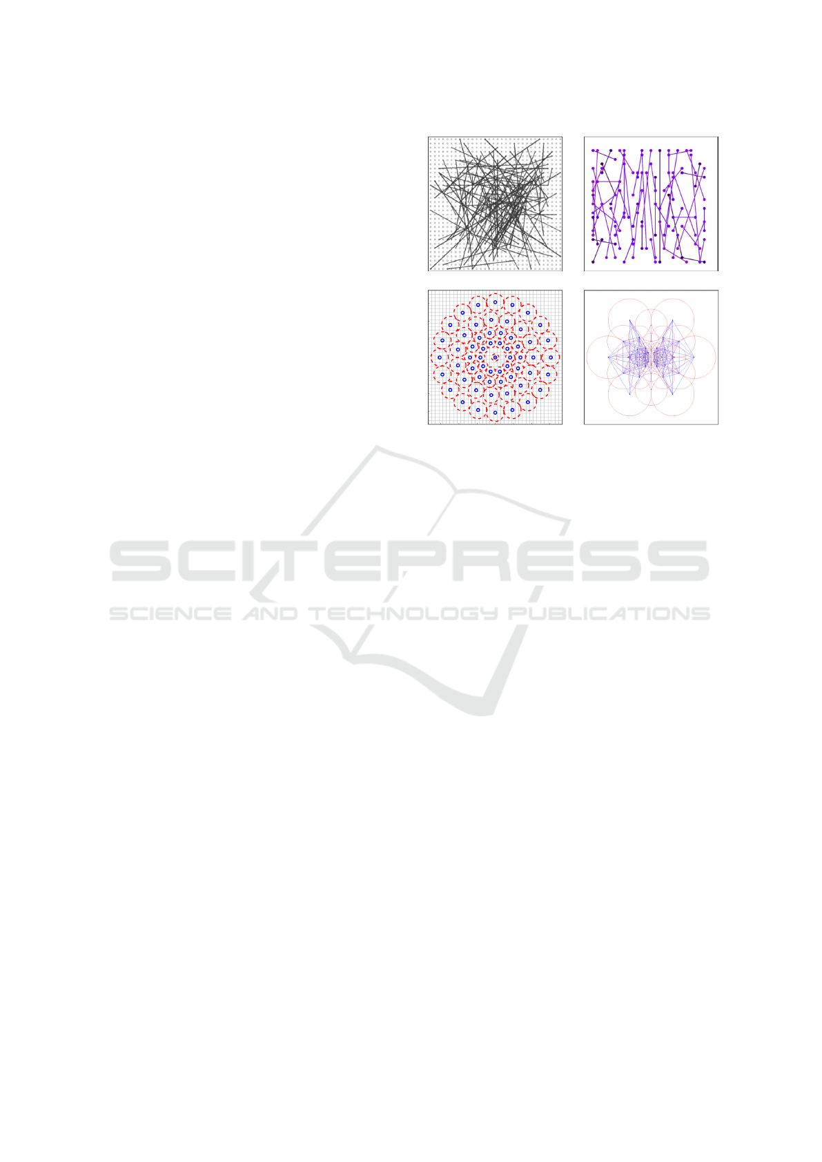
and fair discriminative representation. Figure 1-a
shows a visualization of the selected binary tests of
the BRIEF descriptor. ORB (Rublee et al., 2011) is
an extension of BRIEF, but its binary tests selections
were developed from statistical properties. Instead of
a random selection, the authors used a greedy search
to select the 256 binary tests with higher variance and
lower correlation, what improved its discrimination
power. Figure 1-b shows a visualization of the ORB
binary tests.
BRISK (Leutenegger et al., 2011) and FREAK
(Ortiz, 2012) are based on fixed sets of points, defi-
ned by their designers. The BRISK’s binary tests are
organized using 60 concentric points, as shown in Fi-
gure 1-c, from which two sets of binary tests are crea-
ted: L (long-distance) and S (short-distance). L set is
used to compute canonical orientation and the S set,
(a) BRIEF (b) ORB
(c) BRISK (d) FREAK
Figure 1: Different spatial distribution used to extract bi-
nary tests: a) BRIEF (Calonder et al., 2010); b) ORB (Ru-
blee et al., 2011); c) BRISK (Leutenegger et al., 2011); and
d) FREAK (Ortiz, 2012). Images extracted from the origi-
nal papers.
containing 512 binary tests, is used to generate the fi-
nal descriptor. FREAK’s binary tests, for their turn,
are based on the human eye, more specifically on hu-
man retina, where light receptor cells concentration is
higher in the central region. From the 43 points and

43
2

= 903 possible pairs, 512 binary tests were se-
lected like ORB greedy search. Figure 1-d shows the
locations of the points and final binary tests used by
FREAK.
Instead of using only pixel intensity, the OSRI
descriptor (Xu et al., 2014) is generated by compa-
ring invariant to rotation and illumination subregions,
which are defined according to pixels intensities and
gradients orientation. To build the final binary vector,
the best bits are selected by a cascade filter. BOLD
descriptors (Balntas et al., 2015) select the best bi-
nary tests by a global and local optimization process.
The global optimization is performed offline, and it
identifies the binary tests with high variance and low
correlation in a total set of N patches. In the local op-
timization, each patch is considered a separate class
and new synthetic instances are generated online to
estimate intra-class variance. This second step selects
the binary tests that minimize the variance.
Most recently, binary descriptors based on Con-
volutional Neural Networks (CNN) are being used in
local feature extraction. Two representative approa-
ches are the DeepBit (Lin et al., 2016) and DBD-MQ
(Duan et al., 2017). They use the 16 pre-trained lay-
VISAPP 2019 - 14th International Conference on Computer Vision Theory and Applications
262

ers of VGG network (Simonyan and Zisserman, 2015)
that is fine-tuned by matching local regions using cor-
responding and non-corresponding patch pairs. In
these works, there is no an exact definition of the bi-
nary tests coordinates, since their general idea is to
learn weights that minimize the quantization error of
the real output vector to bits 0 and 1. Despite the qua-
lity of their results, binarizing the last layer maintains
a high computational cost. In this paper, we evalu-
ated CNN ability in binary tests selection, aiming to
discovery different spatial distributions to create dis-
criminant descriptors.
3 METHODOLOGY
3.1 Convolutional Neural Network
Based on the Network proposed by (Simo-Serra et al.,
2015), we built a Convolutional Neural Network with
4 layers. The first three layers consist of blocks of
convolution, pooling and activation function, and the
last layer is fully connected that outputs the coordina-
tes θ
i
of binary tests for each patch p
i
.
The first layer contains 32 convolution kernels of
size 7 × 7, followed by a 2 × 2 max pooling window
and activation function tanh. The second layer is
composed of 64 convolution kernels 6 × 6, followed
by a 3 ×3 max pooling window and activation tanh. In
the third layer, we used 128 convolution kernels 5× 5,
a 4 × 4 max pooling window and activation function
tanh. The fourth layer has no convolution neither
pooling, but only the weights of each processing unit
and the activation function sigmoid. The activation
function is applied to limit the output inside the inter-
val (0, 1), which allows to scale easily to the interval
[
0, S
]
multiplying θ
i
by S, where S × S is the size of
a training patch p
i
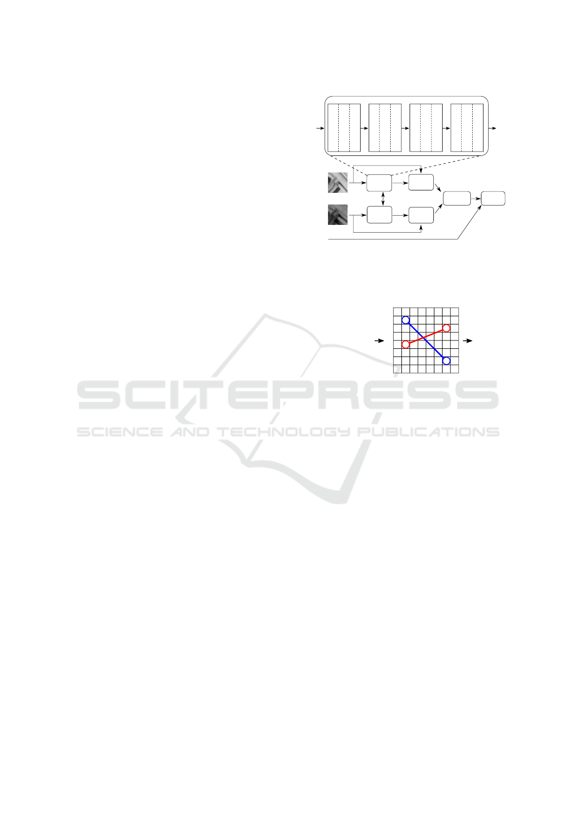
. Figure 2 shows a visualization of
the CNN structure. The final network contains a total
of 805, 632 parameters.
To learn the binary tests, we created a Siamese
Network using 2 CNNs with the aforementioned ar-
chitecture. They share all weights W
i
and bias b
i
,
allowing to train them with patch pairs. Figure 2
illustrates the architecture. Since we aim to mini-
mize the distance between corresponding and maxi-
mize the distances between non-corresponding patch
descriptors, we added the layers d
i
(p
i
, θ
i
), H(d
1
, d
2
)
and L(H, y) to the Siamese Network. Layer d
i
(p
i
, θ
i
)
computes the binary descriptor from the coordina-
tes θ
i
generated by patch p
i
. H(d
1
, d
2
) calculates
the Hamming distance between the descriptors d
1
and d
2
. Finally, L(H, y) computes the error using
ContrastiveLoss function (Simo-Serra et al., 2015),
CNN A
CNN B
d
1
(x
1
,θ
1
)
H(d
1
,d
2
)
W
θ
1
θ
2
d
2
(x
2
,θ
2
)
x
2
x
1
Patches
Siamese Network
L(H, y)
x
i
Conv. (7x7x32)
Pooling (2x2)
Activ. (tanh)
Layer 1
θ
i
Conv. (6x6x64)
Pooling (3x3)
Layer 2
Conv. (5x5x128)
Pooling (4x4)
Layer 3
Fully Connected
Scale to [0,S]
Activ. (sigmoid)
Layer 4
Conv. Network
Activ. (tanh)
Activ. (tanh)
y
Figure 2: Convolutional Network and Siamese Network ar-
chitectures. The Siamese Network is composed of 2 Convo-
lutional Networks that share W
i
and b
i
weights and support
the processing of patches pairs. For each patch p
i
, a coor-
dinates vector θ
i
is generated.
θ = (1, 1, 6, 6, 4, 1, 2, 6)
05 05 10 10 13 01 01 01
0 1 2 3 4 5 6 7
0
1
2
3
4
5
6
7
05 05 11 10 10 01 01 01
05 05 06 09 10 10 01 01
06 06 05 05 25 25 25 25
06 06 05 05 05 25 25 25
25 24 26 05 05 25 25 26
24 24 26 05 03 07 26 26
15 15 15 15 14 10 10 26
d = (1, 0)
(b)
(a) (c)
Figure 3: Representation of the θ vector for a 2-bits binary
descriptor d. a) An instance of the θ vector, θ ∈ N
8
. b) Bi-
nary tests visualization on a 8 ×8 patch. c) Resulting binary
descriptor d from pixel intensities comparison of the binary
tests.
defined as
L(H, y) =
(
H
2
if y = 1,
max(0, C − H)
2
if y = 0,
(2)
where y ∈
{
1, 0
}
is a binary variable that defines if a
patch pair is corresponding (1) or non-corresponding
(0). Equation 2 can be rewritten as
L(H, y) = y · H
2
+ (1 − y) · max(0, C − H)
2
(3)
for implementation convenience. The C constant de-
fines the minimum H distance for descriptors of non-
corresponding patches, penalizing smaller values. In
contrast, the distances between corresponding patches
should be minimized to 0.
3.2 Binary Tests
Given a patch p
i
of size S × S extracted from a digi-
tal image I, a binary test τ(p
i
, x, y, w, z) is a function
that compares pixels p
i
(x, y) and p
i
(w, z) intensities.
Therefore, 4 coordinates are required for each binary
test. To represent a binary descriptor d with n bits,
Exploring the Limitations of the Convolutional Neural Networks on Binary Tests Selection for Local Features
263

the fourth layer of each CNN has been configured to
provide a vector θ
i
∈ N
4
, where 0 ≤ θ
i
≤ S. Figure 3 il-
lustrates an instance of θ for a 2-bits binary descriptor.
The coordinates (1, 1, 6, 6) form the first binary test,
whose result is 1 because pixel intensity p
i
(1, 1) = 05
is less than pixel intensity p
i
(6, 6) = 26 and, likewise,
the coordinates (4, 1, 2, 6) of second binary test results
in 0 because p
i
(4, 1) = 06 is not less than p
i
(2, 6) = 01.
3.3 Gradient
The back-propagation algorithm, used to to update the
weights W
i
and b
i
, depends on the gradient ∇
i
L =
n
∂L
∂W
i
,
∂L
∂b
i
o
of loss function L. Since a Neural Net-
work is a composite function, it is possible to calcu-
late its gradients using the chain rule by equations
∂L
∂W
i
=
∂L
∂H

∂H
∂d
1
∂d
1
∂θ
1
∂θ
1
∂W
i
+
∂H
∂d
2
∂d
2
∂θ
2
∂θ
2
∂W
i

(4)
and
∂L
∂b
i
=
∂L
∂H

∂H
∂d
1
∂d
1
∂θ
1
∂θ
1
∂b
i
+
∂H
∂d
2
∂d
2
∂θ
2
∂θ
2
∂b
i

. (5)
Each training patch pair provides a partial deriva-
tive
∂L
∂H
indicating the direction to modify the Ham-
ming distance and reduce total error. For correspon-
ding patches
∂L
∂H
> 0 when H(d
1
, d
2
) > 0, what me-
ans the Hamming distance must decrease. For non-
corresponding patches
∂L
∂H
< 0 when H(d
1
, d
2
) < C,
indicating that the network must try to increase the
distance to be greater than C. In the previous layer,
the derivatives
∂H
∂d
1
and
∂H
∂d
2
indicate which bits of cur-
rent binary descriptors d
1
and d
2
must be modified
to follow the direction indicated by
∂L
∂H
. Likewise,
the derivatives
∂d
1
∂θ
1
and
∂d
2
∂θ
2
indicate the directions to
change binary tests coordinates θ
1
and θ
2
to modify
the bits indicated by
∂H
∂d
1
and
∂H
∂d
2
. Furthermore, the
derivatives
∂θ
1
∂W
i
,
∂θ
2
∂W
i
,
∂θ
1
∂b
i
and
∂θ
2
∂b
i
indicate the upda-
ting directions of the W
i
and b
i
weights so that the
pixels indicated by
∂d
1
∂θ
1
and
∂d
2
∂θ
2
are selected.
Partial derivatives
∂L
∂H
and
∂θ
i
∂W
i
can be calculated
analytically but
∂H
∂d
i
and
∂d
i
∂θ
i
cannot because they de-
pend on non-differentiable operations, such as Exclu-
sive OR and pixels intensities comparison. Thus, we
approximate
∂L
∂θ
i
numerically by finite differences as
follows. First we define
L
+
1
= L(H(d
1
(x
1
, θ
1
+ ∆), d
2
(x
2
, θ
2
)), y), (6)
L
−
1
= L(H(d
1
(x
1
, θ
1
− ∆), d
2
(x
2
, θ
2
)), y), (7)
0 1 2 3 4 5 6 7
0
1
2
3
4
5
6
7
0 1 2 3 4 5 6 7
0
1
2
3
4
5
6
7
0 1 2 3 4 5 6 7
0
1
2
3
4
5
6
7
0 1 2 3 4 5 6 7
0
1
2
3
4
5
6
7
(a) (b) (c)
0 1 2 3 4 5 6 7
0
1
2
3
4
5
6
7
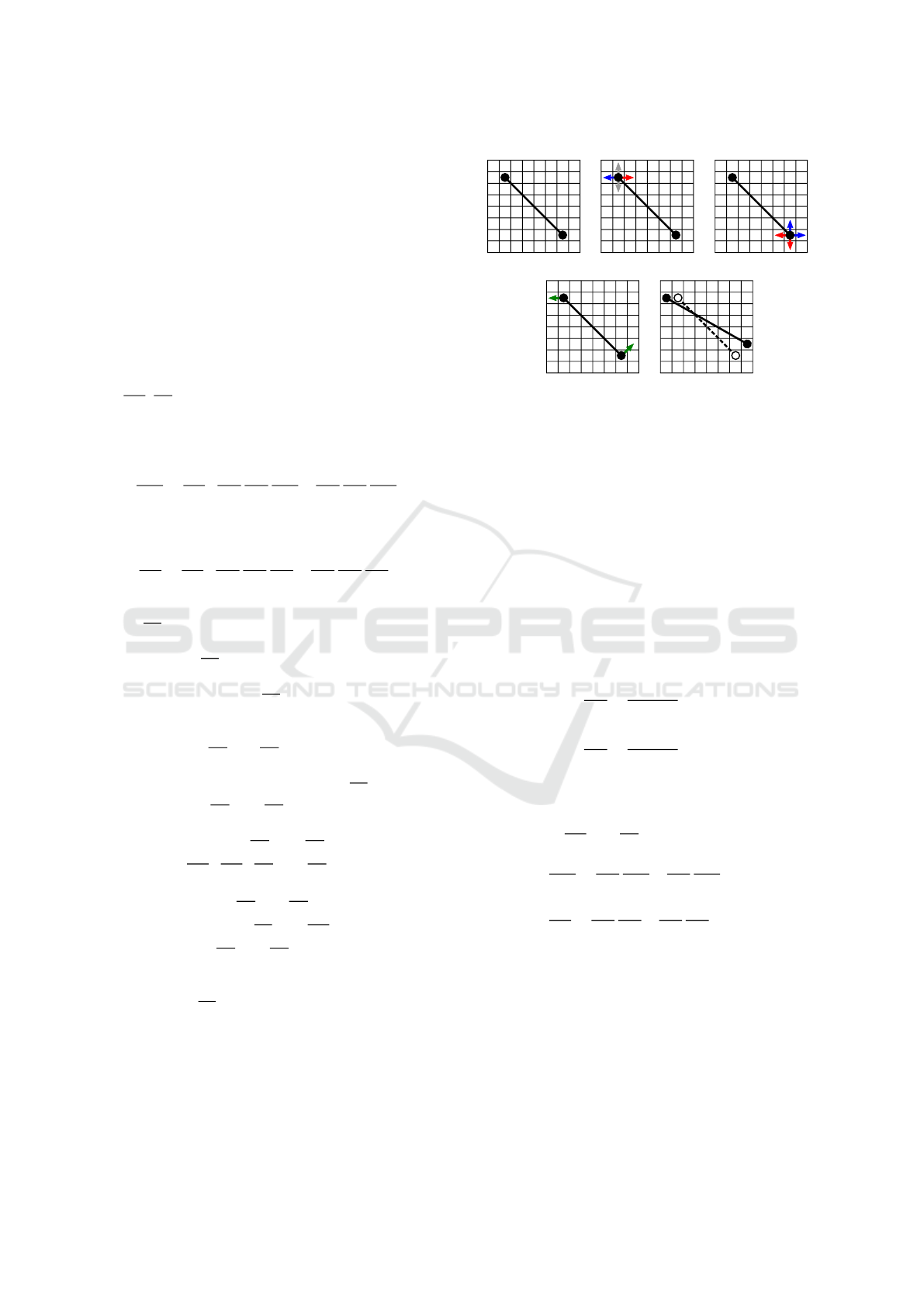
(d) (e)
Figure 4: Illustration of binary tests selection process. a)
One binary test θ = (x
1
, y
1
, x
2
, y
2
) on a patch of size 8 × 8;
b) and c) the error on horizontal e vertical directions when
changing coordinates x
1
, y
1
, x
2
and y
2
. Blue arrows indi-
cate the error decreases, red arrows indicate the error incre-
ases and gray arrows indicate the error does not change. d)
Green arrows indicate the resulting directions when chan-
ging coordinates x
1
, y
1
, x
2
and y
2
after error computation;
e) Resulting binary test after updating network weights.
L
+
2
= L(H(d
1
(x
1
, θ
1
), d
2
(x
2
, θ
2
+ ∆)), y), (8)
L
−
2
= L(H(d
1
(x
1
, θ
1
), d
2
(x
2
, θ
2
− ∆)), y), (9)
then, using the centralized formula we obtain
∂L
∂θ
1
=
L
+
1
− L
−
1
2δ
, (10)
∂L
∂θ
1
=
L
+
2
− L
−
2
2δ
. (11)
In terms of pixels coordinates, we have min δ =
1 for the original image resolution and ∆ =
(δ
1
, δ
2
, ..., δ
N
), where δ
i
= 1 and N = 4 · #bits. Thus,
the gradients
∂L
∂W
i
and
∂L
∂b
i
were calculated as
∂L
∂W
i
=
∂L
∂θ
1
∂θ
1
∂W
i
+
∂L
∂θ
2
∂θ
2
∂W
i
, (12)
∂L
∂b
i
=
∂L
∂θ
1
∂θ
1
∂b
i
+
∂L
∂θ
2
∂θ
2
∂b
i
(13)
instead of using Equations 4 and 5.
Applying this formulation, the Siamese Network
changes the pixels coordinates in horizontal and ver-
tical directions to choose binary tests that decrease the
total error. This is done by selecting binary tests that
reduces the Hamming distance between descriptors of
the corresponding patch pairs and increase the Ham-
ming distance between non-corresponding pairs. Fi-
gure 4 illustrates the coordinates variation process and
the resulting binary test.
VISAPP 2019 - 14th International Conference on Computer Vision Theory and Applications
264

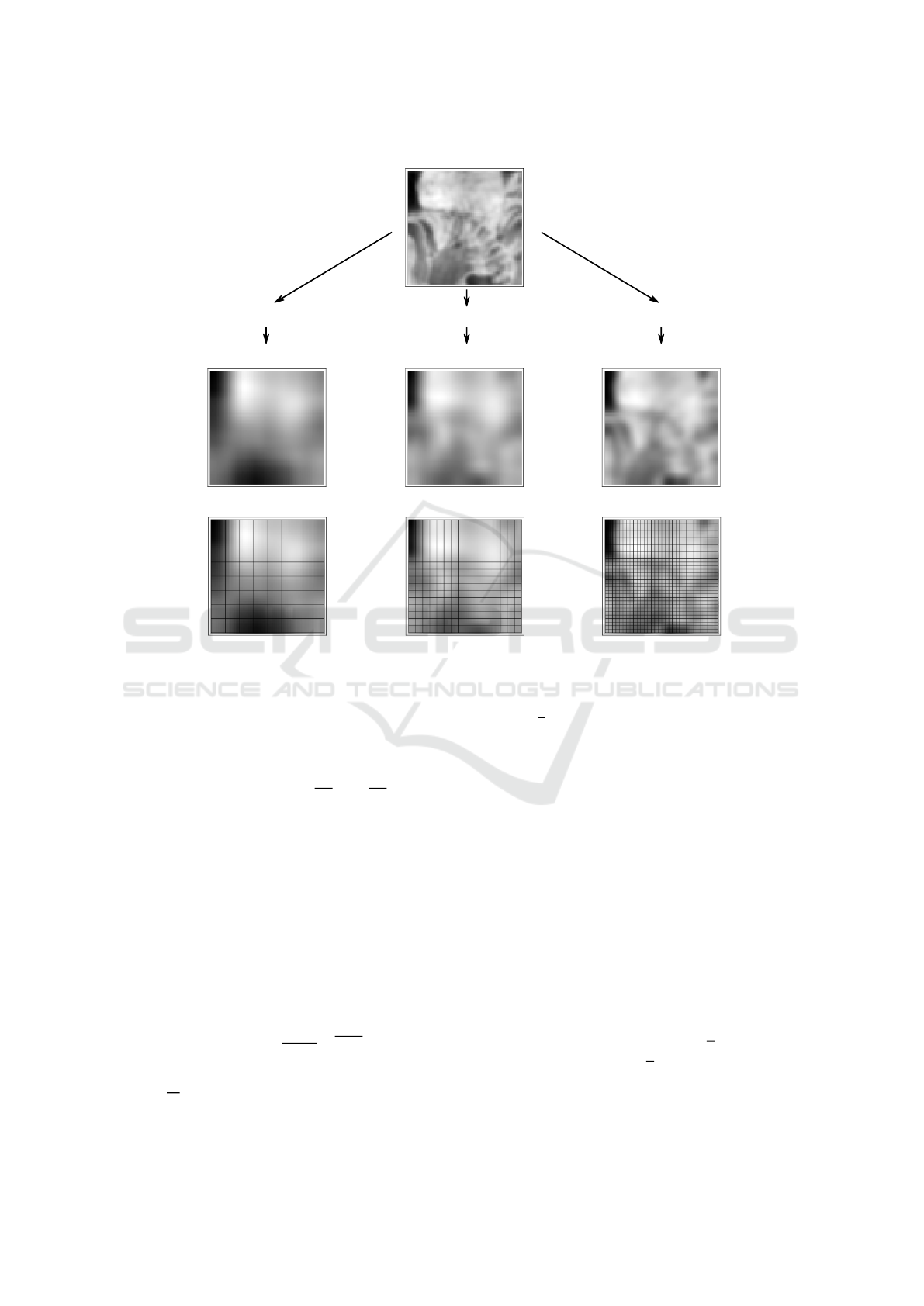
8x8 Resolution
G(x, y; k=25, σ=10)
G(x, y; k=13, σ=5,2)
G(x, y; k=7, σ=2,8)
64x64 Resolution
Grid over patches
16x16 Resolution 32x32 Resolution
8x8 Grid 16x16 Grid 32x32 Grid
Rescaled patches
Figure 5: Patch 64 × 64 rescaled with Gaussian filters G(x, y; k, σ) to 8 × 8, 16 × 16 and 32 × 32 resolutions. A r × r grid
corresponding to the current resolution r is applied to ensure the spatial distribution of the binary tests over the rescaled
patches. In this case, binary tests can be composed of only the central pixels of each grid block.
3.4 Multiscale Trainning
After running experiments using binary tests repre-
sentation described in subsection 3.2 and the numeri-
cal approximation of gradients
∂L
∂θ
1
and
∂L
∂θ
2
, we dis-
covered that the Siamese Network reached local mi-
nimum during training. This local minimum enforces
the network to stop learning before the error becomes
satisfactorily low. Section 4 presents the details and
thorough analysis of the local minimum problem.
To reduce the impacts of local minimum, we trai-
ned the network using image pyramid, from lowest re-
solution to highest. This approach allows the Siamese
Network to view whole patches and select discrimi-
native regions before choosing specific binary tests.
Scale reduction was performed by applying convolu-
tions with a Gaussian filter
G(x, y; k, σ) =
1
2πσ
2
e
−
x
2
+y
2
2σ
2
, (14)
where k × k are the dimensions of kernel, computed
as k =

3S
r
+ 1

, S × S the dimensions of patch, r the
spatial resolution for which patches will be reduced
and σ =
k
f
. In our experiments, we used f = 2.5 to
cover 98.76% of Gaussian kernel.
4 EXPERIMENTS
We performed several experiments to evaluate the net-
work behavior when selecting the binary tests. We
used patches of 64 × 64 size extracted from the da-
taset Trevi Fountain (Winder and Brown, 2007) to
compose corresponding and non-matching pairs. The
Trevi Fountain dataset contains more than 30, 000
keypoints, each one containing between 5 and 50 in-
stances (patches) captured under rotation, scale, and
illumination changes.
To improve the generalization capacity, we enfor-
ced an uniform selection of patches by assigning to
each keypoint the quotas Q
cp
=

P ·
T
k

of correspon-
ding pairs and Q
np
=

N ·
T
k

of non-matching pairs.
These quotas are based on total amount T of patch
pairs to be created, k amount of available keypoints
for trainning and on desired percentages P ∈ [0, 1] and
Exploring the Limitations of the Convolutional Neural Networks on Binary Tests Selection for Local Features
265

Epoch 0 Epoch 10 Epoch 20 Epoch 30
Corresponding
pairs
Non-corresponding
pairs
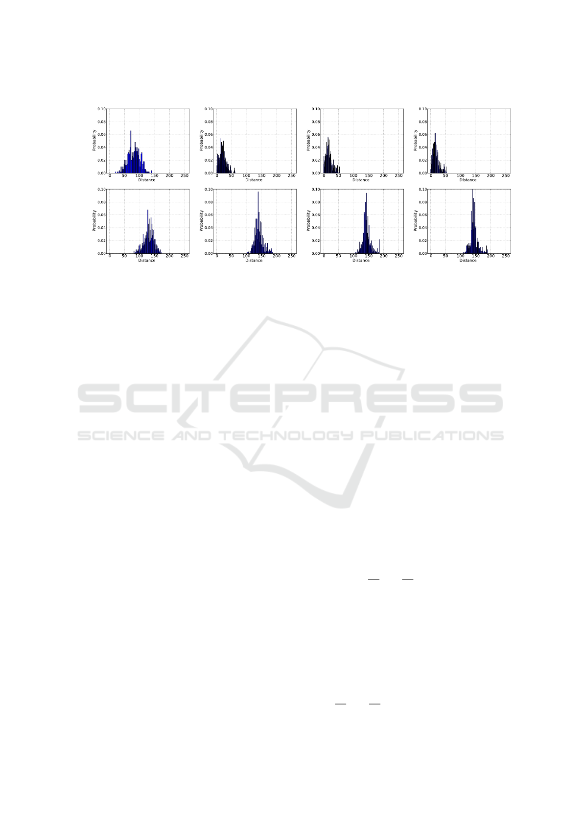
Figure 6: Distribution of distances between correspondent and non-correspondent pairs during Siamese Network Training.
The results of Epoch 0 are before the beginning of the training phase, with random W
i
and b
i
weights. One can clearly see that
the distances of the correspondent pairs decreased over the training, while non-correspondent distances concentrate around
the 125 value. This behavior demonstrates the correct learning of the binary tests.
N = 1 − P of corresponding and non-corresponding
pairs, respectively. Thus, at least two patches of each
keypoint are used.
The siamese network was trained using the K-
Fold protocol, with K = 5. Three folds were used
for training, one for validation and one for testing.
We created T = 10, 000 patch pairs per fold, where
50% were corresponding and 50% non-corresponding
pairs. The network was trained with a total of 30, 000
pairs. For optimization we used the Stochastic Gra-
dient Descent (SGD) algorithm, with batch size 32,
learning rate 1 × 10
−9
, momentum 0.9 and decay
1 × 10
−3
. We performed 30 training epochs because
decreasing error rate stagnates after this value. In
objective function, i.e., contrastive loss, the best re-
sult was obtained using margin C = 150. Our mo-
del were implemented in Python with Keras (Chollet
et al., 2015) and Theano (Theano Development Team,
2016) libraries.
4.1 Distances Distributions
The distance distributions indicate whether network
learning of binary tests is occurring as expected. Ide-
ally, distances between corresponding patch descrip-
tors should be close to zero, and distances between
non-corresponding descriptors should be large, accor-
ding to the applied similarity measure.
We performed this analysis observing distances
every 10 training epochs, where epoch 0 refers to the
initial state of Siamese Network, with weights rand-
omly initialized. Figure 6 presents the histograms
of distances that demonstrate the expected behavior
because the distances between corresponding patch
descriptors were reduced while the distances between
non-corresponding descriptors increased during trai-
ning. In the first row, one can observe distances be-
tween corresponding patch descriptors moving to the
left side while distances between non-corresponding
patch descriptors go to the right side and stop around
150.
4.2 Local Minima
Binary tests selection based on the local pixel’s neig-
hborhood is limited by Local Minima problem due
to the spatial distribution of pixels intensities. At the
beginning of the training step, until epoch 10, hori-
zontal and vertical variations of coordinates θ
i
reduce
the error, but after some epochs, the immediate neig-
hbors θ
i
+ ∆ and θ
i
− ∆ do not change order relation
between pixels of the current binary tests. It means
the resulting bits remain the same when the network
change coordinates in directions right, left, up, and
down.
This finding is the result of analyzing the distribu-
tions of vectors
∂L
∂θ
1
and
∂L
∂θ
2
components throughout
the training. They point to directions that reduce the
error in the optimization space. Components with po-
sitive values indicate that the error decreases by mo-
ving that binary test to left or up directions and com-
ponents with negative values indicate that the error
decreases by moving that binary test to right or down
directions. Components equal to 0 suggest that the
error does not change in that direction.
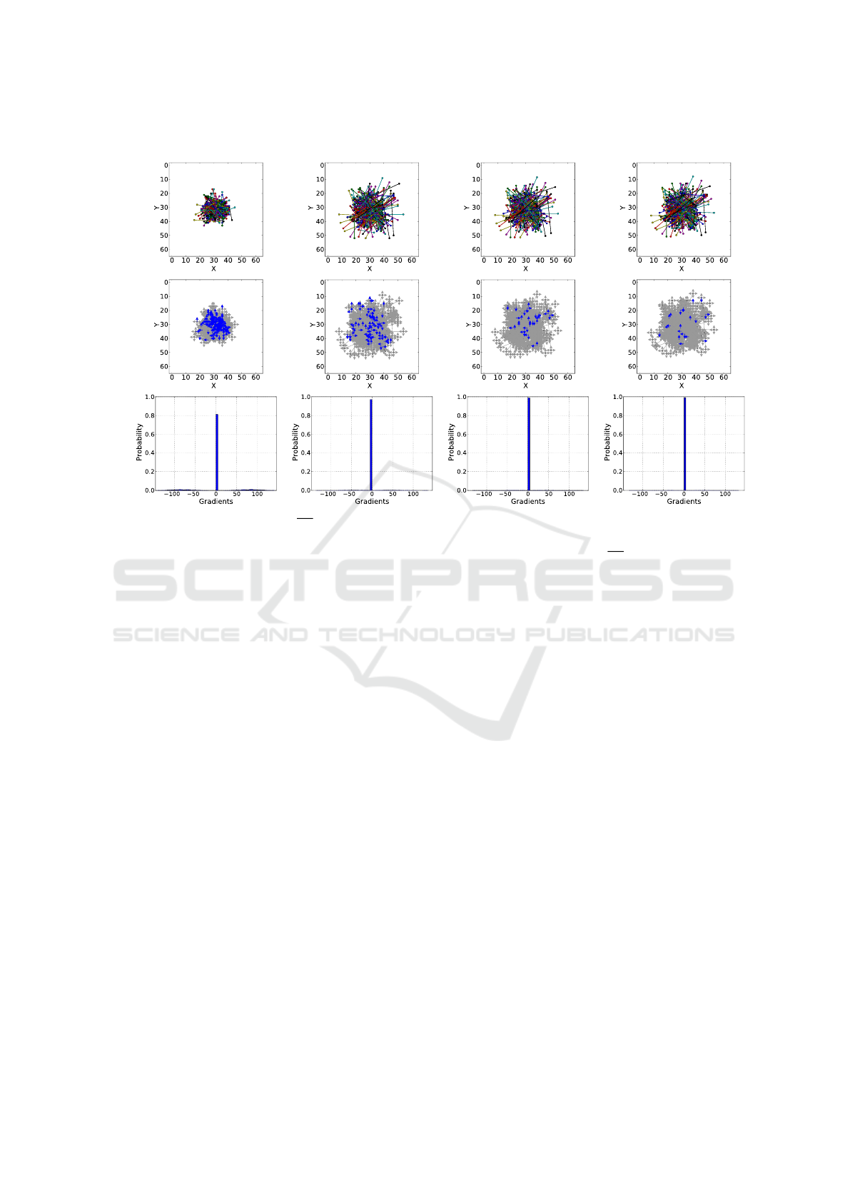
Figure 7 presents the binary tests of an instance
patch together with visualizations and distributions of
vectors
∂L
∂θ
1
and
∂L
∂θ
2
components throughout 30 trai-
VISAPP 2019 - 14th International Conference on Computer Vision Theory and Applications
266

Epoch 0 Epoch 10 Epoch 20 Epoch 30
Ditribution of
Gradients
Binary tests
gradient components
Figure 7: Visualization of gradients
∂L
∂θ
i
components demonstrating the existence of local minima. The results of Epoch 0
were generated before training starts, with random weights. Images in the top row show the binary tests of an instance patch
during training. Images in the mid row show for each selected pixel the directions of its gradients
∂L
∂θ
i
. Blue arrows represent
values different from 0 (positive or negative) and indicate the directions to reduce error. Gray arrows represent values equal to
0 and indicate the error keeps the same in those directions and orientations. The bottom row shows the distributions of gradient
components, where one can observe the concentration at 0 increases during training, making the network stops learning.
ning epochs. Results of epoch 0 refer to the initial
state of the Siamese Network, with weights W
i
and
b
i
randomly initialized, for comparison and analysis.
One can see at the first row a spreading of binary tests
until the epoch 10 due to the existence of non-zero
components (positive or negative) in the gradients, re-
presented by blue arrows at the second image row.
Gray arrows represent zero components. Histograms
in the third row show a strong concentration of com-
ponents equal to 0, which means that binary tests will
not change anymore and learning has stagnated.
4.3 Impact of Multiscale Trainning
The Local Minimum problem appears because the se-
lection of binary tests was made by analyzing only
immediate neighbors of current pixels. This localized
view hinders the selection of further pixels and stag-
nates the network learning after a few training epochs.
To reduce impacts of Local Minimum, we propose
to use a multi-scale training, changing patches reso-
lutions after some epochs by applying convolutions
with Gaussian kernels. All details of this step are pre-
sented in Section 3.4.
Spatial resolution 8 × 8 was simulated convolving
all patches with a Gaussian kernel G(x, y; k = 25, σ =
10) and dividing them in a regular grid 8 × 8 formed
by cells of size 8 × 8 pixels. Resolution 16 × 16 was
simulated with a Gaussian kernel G(x, y; k = 13, σ =
5, 2) and a grid 16 × 16 formed by cells of size 4 ×
4 pixels. We also simulated resolution 32 × 32 with
a Gaussian kernel G(x, y; k = 7, σ = 2, 8) and a grid
32 × 32 of size 2 × 2 pixels.
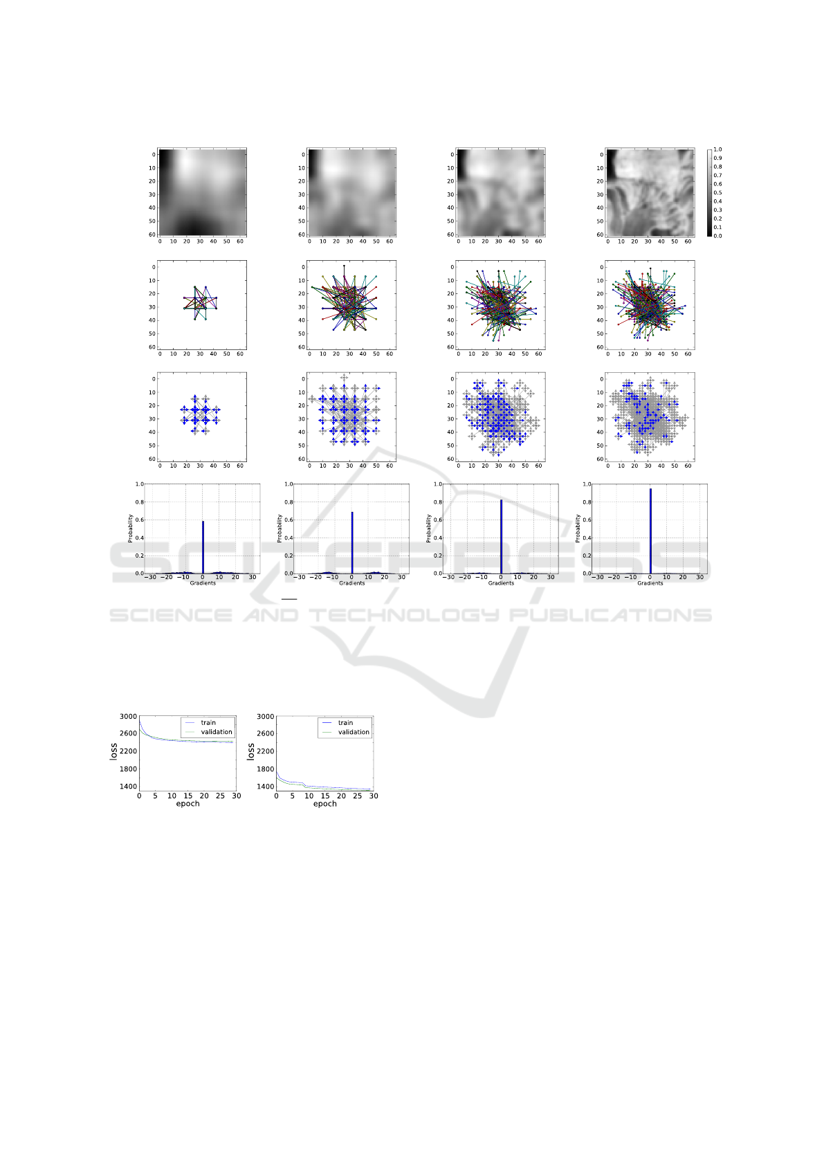
By constraining the selection on central pixels of
each grid cell, at respective resolution, binary tests be-
came more spread than initial version of training, as
shown in Figure 8. In the first row we show an in-
stance patch varying scale every 10 epochs, starting
from resolution 8 × 8, to 16 × 16, then 32 × 32 and fi-
nally 64 × 64 (the original resolution). In the second
row we show the binary tests for the displayed patch,
where one can observe the regularity of the selected
pixels over the grid. At the third row, we show the
gradients (colored arrows) of binary tests in its speci-
fic resolution. Blue arrows indicate non-zero compo-
nents while gray arrows indicate components equal to
0. Finally, the fourth row presents the gradient com-
ponents distributions.
Comparing the gradients and histograms in Figu-
res 7 and 8, one can observe a significant reduction of
Exploring the Limitations of the Convolutional Neural Networks on Binary Tests Selection for Local Features
267

Patch in different
Binary tests
Gradients
scales
Distribution of
gradient components
Epoch 0
Epoch 10
Epoch 20
Epoch 30
Figure 8: Visualization of gradients
∂L
∂θ
i
components in multi-scale training illustrating the reduction of Local Minima. Epoch
0 results were generated before any training, with random weights, for comparison purposes. Figures in the first row show
an instance patch varying scale during training. The second row shows the binary tests learned for the patch shown above.
Third-row show for each selected pixel the directions of its gradients. Blue arrows represent values different from 0 (positive
or negative) and indicate the directions to reduce error. Gray arrows represent values equal to 0 and indicate the error keeps
the same in those directions and orientations. The last row shows the distributions of gradient components, where one can
observe the concentration in 0 was reduced compared of Figure 7.
(a) (b)
Figure 9: Error histories in different binary tests learning
experiments. a) Trained with patches in the original 64 × 64
scale. b) Trained with 8 ×8 scale until epoch 10, then chan-
ged to 16 × 16 scale, learning rate 1 × 10
−9
. It is possible
to observe a significant decreasing in the loss value, espe-
cially when the scale is changed, which demonstrates that
the proposed approach was able to lessen the Local Minima
problem.
zero components since the beginning of training. That
means the Siamese Network found more pixels to re-
duce the error. At epoch 0 of Figure 7 there were more
than 80% of gradient components equal to 0 while Fi-
gure 8 shows less than 60% at the same time. On
epoch 10 of Figure 7 components equal to 0 excee-
ded 90% whereas at the same time in Figure 8 this
concentration was still less than 70%.
The multiscale trainning allows the network to ex-
pand on the covered area over all patches, making
possible to select further pixels to form binary tests.
We obtained the best result by starting the training pa-
tches at spatial resolution 8 × 8 and, after 10 epochs,
changing to resolution 16 × 16. Figure 9 shows the
error curves for the train and validation, comparing
standard and multiscale training. Figure 9-a shows
that the error started close to 2, 900 at epoch 0 and
stabilized around 2, 400 after 30 epochs. Figure 9-b
shows that the error started close to 1, 700 and became
close to 1, 300 after 30 epochs. From these results we
draw the following observation: the proposed appro-
VISAPP 2019 - 14th International Conference on Computer Vision Theory and Applications
268

A
B
C
(a) (b) (c)
Figure 10: Illustration of the Incorrect Gradient Components problem. a) Some fictitious binary tests selected during the
training. b) Visualization of gradients
∂L
∂θ
i
components. Arrows represent the loss values behavior given a coordinates θ
i
variation of the binary tests in either vertical or horizontal axes. Blue indicates a decrease of the loss value in that direction,
red indicates an increase of the loss value and gray indicates no change of the loss value. c) Green arrows indicate the resulting
directions that should be followed by the Siamese Network weight update. Vectors A, B, and C are the Incorrect Gradient
Components, since their directions do not decrease the loss value. They are obtained from individual components that either
increase or do not modify the loss value.
ach has reduced the impact of Local Minimum, alt-
hough it was not completely solved.
EdgeFoci Webcam Viewpoints
Figure 11: Sample images from Viewpoints (Yi et al.,
2016), Webcam (Yi et al., 2016) and EdgeFoci (Ramnath
and Zitnick, 2011) datasets.
4.4 Incorrect Gradient Components
The selection of the binary tests based on the imme-
diate pixels neighbors also presents a problem rela-
ted to some components of the gradient vectors
∂L
∂θ
1
and
∂L
∂θ
2
. The gradient vector ∇ f (x) indicates the di-
rection and orientation of the greatest rate of increase
of the function f (x) from x. To minimize f (x), the
Gradient Descent algorithm updates weights W
i
and
b
i
following the gradient direction but in the oppo-
site orientation, what is valid when f (x) is a convex
function and the opposite orientation to greatest rate
of increase is precisely the one that gives the largest
decreasing rate of f (x) at x. We discovered it is not
true for the binary tests selection problem.
We also have found that the Siamese Network
changes the coordinates of some binary tests not be-
cause the neighbor might reduced the error, but sim-
ply because the gradients
∂L
∂θ
1
and
∂L
∂θ
2
indicate that
the function L(H, y) grew up in the opposite orienta-
tion. This problem of the learning going to the wrong
way to minimize the loss function we called Incorrect
Components of Gradient Problem.
The gradient
∂L
∂θ
1
has incorrect components when
the inequalities
L
+
1
≥ L(H(d
1
(x
1
, θ
1
), d
2
(x
2
, θ
2
)), y) and (15)
L
−
1
≥ L(H(d
1
(x
1
, θ
1
), d
2
(x
2
, θ
2
)), y) (16)
are true simultaneously. Similarly, the gradient
∂L
∂θ
2
contains incorrect components when
L
+
2
≥ L(H(d
1
(x
1
, θ
1
), d
2
(x
2
, θ
2
)), y) and (17)
L
−
2
≥ L(H(d
1
(x
1
, θ
1
), d
2
(x
2
, θ
2
)), y). (18)
The terms L
+
1
, L
−
1
, L
+
2
and L
−
2
are defined in Eq. 6,
7, 8 and 9. Figure 10 illustrates the components of
the gradients
∂L
∂θ
1
and
∂L
∂θ
2
for a fictional patch 18 × 18,
where it is possible to visualize the resulting vectors
used by the Siamese Network to update the weights
W
i
and b
i
.
4.5 Descriptor Evaluation
To evaluate the proposed binary tests selection met-
hodology, we performed keypoint matchings experi-
ments using images of the datasets Viewpoints (Yi
Exploring the Limitations of the Convolutional Neural Networks on Binary Tests Selection for Local Features
269

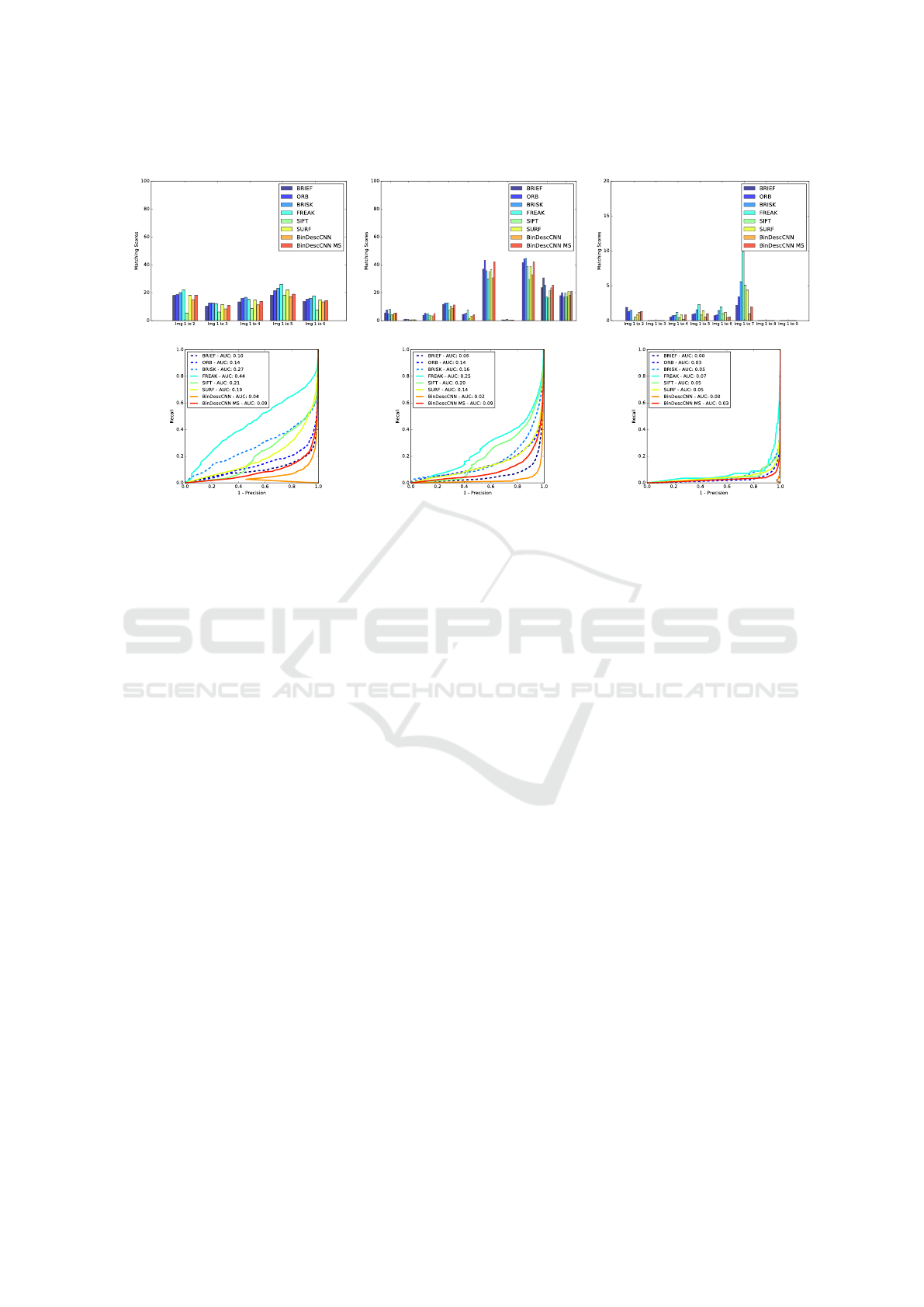
1-Precision x Recall Matching Score
Viewpoints Webcam EdgeFoci
Scene: Posters Scene: Courbevoie Scene: Obama
Img 1 to 2 Img 1 to 2 Img 1 to 2
Img 1-2 Img 1-3 Img 1-4 Img 1-5 Img 1-6 Img 1-7 Img 1-8 Img 1-9 Img 1-10
Img 1-11
Figure 12: Qualitative evaluation of binary tests learned by the Siamese Network. BinDescCNN descriptor represents our
model trained on Trevi Fountain dataset with patches in original scale 64 × 64 while BinDescCNN MS were trained with
patches in scales 8 × 8 and 16 × 16.
et al., 2016), Webcam (Yi et al., 2016), and EdgeFoci
(Ramnath and Zitnick, 2011). Each dataset is compo-
sed of different images of several scenes. Figure 11
shows some samples of images from the datasets.
Dataset Viewpoints is composed of 30 images in
total, divided into 5 different sequences. Each se-
quence was created from images captured with pose
variations. Some of these images have also scale va-
riations. Dataset EdgeFoci contains 38 images divi-
ded into 5 sequences with different poses and lighting
variations. Webcam has 120 images divided into 6
sequences with lighting variations. The images were
acquired with the camera in a fixed position throug-
hout the day in different seasons.
We first evaluate the quality of the descriptor in
a matching task. We used a Matching Score defined
as the fraction of correctly matched keypoints bet-
ween two images. We evaluated two models: Bin-
DescCNN that was trained with patches of the data-
set Trevi Fountain in original resolution 64 × 64; and
the BinDescCNN MS that was trained with multi-scale
patches, as described in subsection 3.4. The BinDes-
cCNN MS model presented better results than BinDes-
cCNN due to a reduction of Local Minimum impacts,
which allowed a better choice of pixels to compose
binary tests. We compared our results against the flo-
ating point descriptors SIFT and SURF and also the
known binary descriptors BRIEF, ORB, BRISK and
FREAK. To avoid any bias, all descriptors were eva-
luated using the ORB algorithm as a keypoint detec-
tor.
We also used the Area Under the Curve (AUC) of
1-Precision × Recall chart. Precision is a measure
of the probability that a sample is correctly classified
when a model says it belongs to a certain class. Re-
call evaluates how many correct samples have been
classified as correct. Figure 12 shows some results
obtained on datasets Viewpoints, Webcam and Edge-
Foci, respectively. In general, our models reached a
Matching Score close to the BRIEF and ORB des-
criptors, but worse than BRISK, FREAK, and SURF.
In this same metric, the SIFT descriptor performance
was poorer than others due to use of ORB as keypoint
detector. We believe that the detected keypoints are
not appropriate to SIFT because their gradients dis-
tributions are not discriminative enough. Results pre-
sented in the curves 1-Precision × Recall show that,
in general, our descriptor is better than BRIEF, howe-
ver demonstrated some confusion when performing
matchings. Despite the reasonable amount of correct
matchings our approach still produces large number
of False Positives and False Negatives.
5 CONCLUSION
In this work, we show that binary tests learned by the
Siamese Network are still a major challenging task for
CNN. Network’s learning stops after a few epochs due
to the Local Minima and Incorrect Gradient Compo-
nents problems, what make difficult to separate cor-
VISAPP 2019 - 14th International Conference on Computer Vision Theory and Applications
270

responding and non-corresponding patches properly.
We conclude that not always a CNN based model
will be able to find a spatial binary tests distribu-
tion to minimize the distances between correspon-
ding keypoints and maximize the distances between
non-corresponding keypoints. The results presented
do not prove the impossibility of using Convolutio-
nal Neural Networks to select binary tests, but they
clarify some limitations when using the local pixel’s
neighborhood.
ACKNOWLEDGEMENTS
The authors would like to thank the agencies CAPES,
CNPq, and FAPEMIG for funding different parts of
this work.
REFERENCES
Balntas, V., Tang, L., and Mikolajczyk, K. (2015). Bold
- binary online learned descriptor for efficient image
matching. In The IEEE Conference on Computer Vi-
sion and Pattern Recognition (CVPR).
Bay, H., Tuytelaars, T., and Gool, L. V. (2006). Surf: Spee-
ded up robust features. In In ECCV, pages 404–417.
Calonder, M., Lepetit, V., Strecha, C., and Fua, P. (2010).
Brief: Binary robust independent elementary features.
In Proceedings of the 11th European Conference on
Computer Vision, pages 778–792.
Chollet, F. et al. (2015). Keras.
Dalal, N. and Triggs, B. (2005). Histograms of oriented
gradients for human detection. In Proceedings of the
2005 IEEE Computer Society Conference on Compu-
ter Vision and Pattern Recognition (CVPR’05) - Vo-
lume 1 - Volume 01, pages 886–893.
Duan, Y., Lu, J., Wang, Z., Feng, J., and Zhou, J.
(2017). Learning deep binary descriptor with multi-
quantization. In The IEEE Conference on Computer
Vision and Pattern Recognition (CVPR).
Leutenegger, S., Chli, M., and Siegwart, R. Y. (2011).
Brisk: Binary robust invariant scalable keypoints. In
Proceedings of the 2011 International Conference on
Computer Vision, pages 2548–2555.
Lin, K., Lu, J., Chen, C.-S., and Zhou, J. (2016). Learning
compact binary descriptors with unsupervised deep
neural networks. In IEEE Conference on Computer
Vision and Pattern Recognition (CVPR).
Lowe, D. G. (2004). Distinctive image features from scale-
invariant keypoints. Int. J. Comput. Vision, pages 91–
110.
Ortiz, R. (2012). Freak: Fast retina keypoint. In Pro-
ceedings of the 2012 IEEE Conference on Computer
Vision and Pattern Recognition (CVPR), pages 510–
517.
Ramnath, K. and Zitnick, C. L. (2011). Edge foci inte-
rest points. In 2011 IEEE International Conference
on Computer Vision (ICCV 2011)(ICCV), pages 359–
366.
Rublee, E., Rabaud, V., Konolige, K., and Bradski, G.
(2011). Orb: An efficient alternative to sift or surf.
In Proceedings of the 2011 International Conference
on Computer Vision, pages 2564–2571.
Simo-Serra, E., Trulls, E., Ferraz, L., Kokkinos, I., Fua, P.,
and Moreno-Noguer, F. (2015). Discriminative lear-
ning of deep convolutional feature point descriptors.
In 2015 IEEE International Conference on Computer
Vision (ICCV), pages 118–126.
Simonyan, K. and Zisserman, A. (2015). Very deep convo-
lutional networks for large-scale image recognition. In
In Proc. of International Conference on Learning Re-
presentations (ICLR).
Theano Development Team (2016). Theano: A Python fra-
mework for fast computation of mathematical expres-
sions.
Winder, S. and Brown, M. (2007). Learning local image
descriptors. In Proceedings of the International Con-
ference on Computer Vision and Pattern Recognition
(CVPR07).
Xu, X., Tian, L., Feng, J., and Zhou, J. (2014). OSRI: A
rotationally invariant binary descriptor. IEEE Trans.
Image Processing, pages 2983–2995.
Yi, K. M., Verdie, Y., Fua, P., and Lepetit, V. (2016). Le-
arning to Assign Orientations to Feature Points. In
Proceedings of the Computer Vision and Pattern Re-
cognition.
Exploring the Limitations of the Convolutional Neural Networks on Binary Tests Selection for Local Features
271