Quantitative Afﬁne Feature Detector Comparison based on Real-World

Images Taken by a Quadcopter

Zolt

an Pusztai

1,2

and Levente Hajder

Geometric Computer Vision Group, Machine Perception Laboratory, MTA SZTAKI, Kende st. 17, Budapest 1111, Hungary

Department of Algorithm and Applications, E

otv

os Lor

and University, P

azm

any P

eter stny. 1/C, Budapest 1117, Hungary

Keywords:

Feature detector, Quantitative Comparison, Afﬁne Transformation, Detection Error, Ground Truth Generation.

Abstract:

Feature detectors are frequently used in computer vision. Recently, detectors which can extract the afﬁne

transformation between the features have become popular. With afﬁne transformations, it is possible to esti-

mate the properties of the camera motion and the 3D scene from signiﬁcantly fewer feature correspondences.

This paper quantitatively compares the afﬁne feature detectors on real-world images captured by a quadcopter.

The ground truth (GT) data are calculated from the constrained motion of the cameras. Accurate and very

realistic testing data are generated for both the feature locations and the corresponding afﬁne transformations.

Based on the generated GT data, many popular afﬁne feature detectors are quantitatively compared.

1 INTRODUCTION

Feature detectors have been studied since the born of

computer vision. First, point-related local detectors

are developed to explore properties of camera mo-

tion and epipolar geometry. Local features describe

only a small area of the image, thus they can be ef-

fectively used to ﬁnd point correspondences, even in

the presence of high illumination, viewpoint change

or occlusion. Afﬁne feature detectors can detect the

local afﬁne warp of the detected point regions. The

afﬁne transformation can be used to solve the basic

task of epipolar geometry (e.g. to detect camera mo-

tion, object detection or 3D reconstruction) using less

correspondences than general point features. This pa-

per deals with the quantitative comparison of afﬁne

feature detectors using video sequences, taken by a

quadcopter, captured in a real-world environment.

Interest feature detectors have been studied in a

long period of computer vision. The well-known Har-

ris (Harris and Stephens, 1988) corner detector or Shi-

Tomasi detector (Shi and Tomasi, 1994) have been

published more than two decades ago. Since then,

new point feature detectors have been implemented,

e.g. SIFT (Lowe, 2004), SURF (Bay et al., 2008),

KAZE (Alcantarilla et al., 2012), BRISK (Leuteneg-

ger et al., 2011) and so on. Correspondences are made

using a feature location and a feature descriptor. The

latter describes the local small area of the feature with

a vector in a compact and distinguish way. These des-

criptor vectors can be used for feature matching over

the successive image. Features, whose descriptor vec-

tors are close to each other, potentially yield a match.

While point-based features estimate only point

correspondences, afﬁne feature detectors can extract

the afﬁne transformations around the feature centers

as well. An afﬁne transformation contains the linear

approximation of the warp around the point corre-

spondences. In other words, this is a 2 by 2 linear

transformation matrix which transforms the local re-

gion of the feature to that of the corresponding fea-

ture. Each afﬁne transformation contains enough in-

formation for estimating the normal vector of the tan-

gent plane at the corresponding 3D location of the fe-

ature. These additional constraints can be used to esti-

mate fundamental matrix, camera movement or other

epipolar properties using less number of features, than

using point correspondences.

The aim of this paper is to quantitatively compare

the feature detectors and the estimated afﬁne transfor-

mations, using real-world video sequences captured

by a quadcopter. The literature of previous work is not

rich. Maybe the most signiﬁcant work was published

by Mikolajczyk et al. (Mikolajczyk et al., 2005). They

compare several afﬁne feature detectors using real-

world images. However, in their comparison, either

the camera has ﬁxed location or the scenes are planar,

thus, the images are related by homographies. The er-

704

Pusztai, Z. and Hajder, L.

Quantitative Afﬁne Feature Detector Comparison based on Real-World Images Taken by a Quadcopter.

DOI: 10.5220/0007372907040715

In Proceedings of the 14th International Joint Conference on Computer Vision, Imaging and Computer Graphics Theory and Applications (VISIGRAPP 2019), pages 704-715

ISBN: 978-989-758-354-4

ror for the afﬁne transformations is computed by the

overlapping error of the related afﬁne ellipses or by

the repeatability score. Even trough the authors com-

pared the detectors using several different noise types

(blur, JPEG compression, light change) we think that

the constraints of non-moving camera or planar scene

yield very limited test cases. A comprehensive study

can be found in (Tuytelaars and Mikolajczyk, 2008),

however the paper does not contain any real-world

test. Recently Pusztai et al. proposed a technique to

quantitatively compare feature detectors and descrip-

tors using a structured-light 3D scanner (Pusztai and

Hajder, 2017). However, the testing data consist of

small objects and rotation movement only. Tareen et

al. (Tareen and Saleem, 2018) also published a com-

parison of the most popular feature detector and des-

criptor algorithms. Their ground-truth (GT) data ge-

neration is twofold: (i) They use the Oxfordian data-

set, that was also applied in the work of (Mikolajczyk

et al., 2005), (ii) they generated test images, including

GT transformations, carried out by different kinds of

afﬁne transformations for the original images: trans-

lation, rotation and scale, and the transformed images

are synthesized by common bilinear interpolation. In

the latter case, the processed images are not taken by

a camera, thus the input data for the comparison is not

really realistic.

The literature of afﬁne feature comparisons is not

extensive, despite the fact that it is an important sub-

ject. Most detectors are compared to others, using

only a small set of images, and parameters tuned to

achieve the best results. In real world applications,

the best parameter set may differ from the laboratory

experience. Thus, more comparisons have to be made

using real-world video sequences and various camera

movements.

In this paper, we show, that the afﬁne invariant

feature detectors can be evaluated quantitatively on

real-world test sequences if images are captured by a

quadcopter-mounted camera. The main contributions

of the paper are twofold: (i) First, the GT afﬁne trans-

formation generation is shown in case of several spe-

cial movements of a quadcopter where afﬁne trans-

formations and corresponding point locations can be

very accurately determined. To the best of our know-

ledge, this is the ﬁrst study in which the ground truth

data is generated using real images of a moving cop-

ter. (ii) Then several afﬁne covariant feature detectors

are quantitatively compared using the generated GT

data. Both point locations and the related afﬁne trans-

formations are examined in the comparison.

The structure of this paper is as follows. First, the

rival methods are theoretically described in Section 2.

Then the ground truth data generation methods are

overviewed for different drone movements and ca-

mera orientations. Section 4 contains the methodo-

logy of the evaluation. The test results are discussed

in Section 5, and Section 6 concludes the research.

2 OVERVIEW OF

AFFINE-COVARIANT

DETECTORS

In this section, the afﬁne transformations and the af-

ﬁne covariant detectors are brieﬂy introduced. The

detectors aim to separately ﬁnd discriminate features

in the images. If a feature is found, then the afﬁne

shape can be determined which is usually visualized

as an ellipse. Figure 1 shows the local afﬁne regions

of a corresponding feature pair in successive images.

The methods to detect discriminate features and their

afﬁne shapes vary from detector to detector. They are

brieﬂy introduced as follows:

Harris-Laplace, Harris-Afﬁne. The methods intro-

duced by (Mikolajczyk and Schmid, 2002) are based

on the well-known Harris detector (Harris and Ste-

phens, 1988). Harris uses the so-called second mo-

ment matrix to extract features in the images. The

matrix is as follows:

M(x) = σ

G(σ

)∗ (1)



(x,σ

) f

(x,σ

) f

(x,σ

)

(x,σ

) f

(x,σ

) f

(x,σ

)



where

G(σ) =

2πσ

exp

−

2σ

(x,σ

) =

∂

∂x

G(σ

) ∗ f (x).

The matrix (M) contains the gradient distribution

around the feature, σ

, σ

are called the differenti-

ation scale and integration scale, respectively. A local

feature point is found, if the term det(M)−λtrace(M)

is higher than a pre-selected threshold. This means

that both of the eigenvalues of M are large, which in-

dicates a corner in the image.

After the location of the feature is found, a cha-

racteristic scale selections needs to be carried out.

The circular Laplace operator is used for this purpose.

The characteristic scale is found if the similarity of

the operator and the underlying image structure is the

highest. The ﬁnal step of this afﬁne invariant detector

is to determine the second scale of the feature points

using the following iterative estimation:

1. Detect the initial point and corresponding scale.

Quantitative Afﬁne Feature Detector Comparison based on Real-World Images Taken by a Quadcopter

705

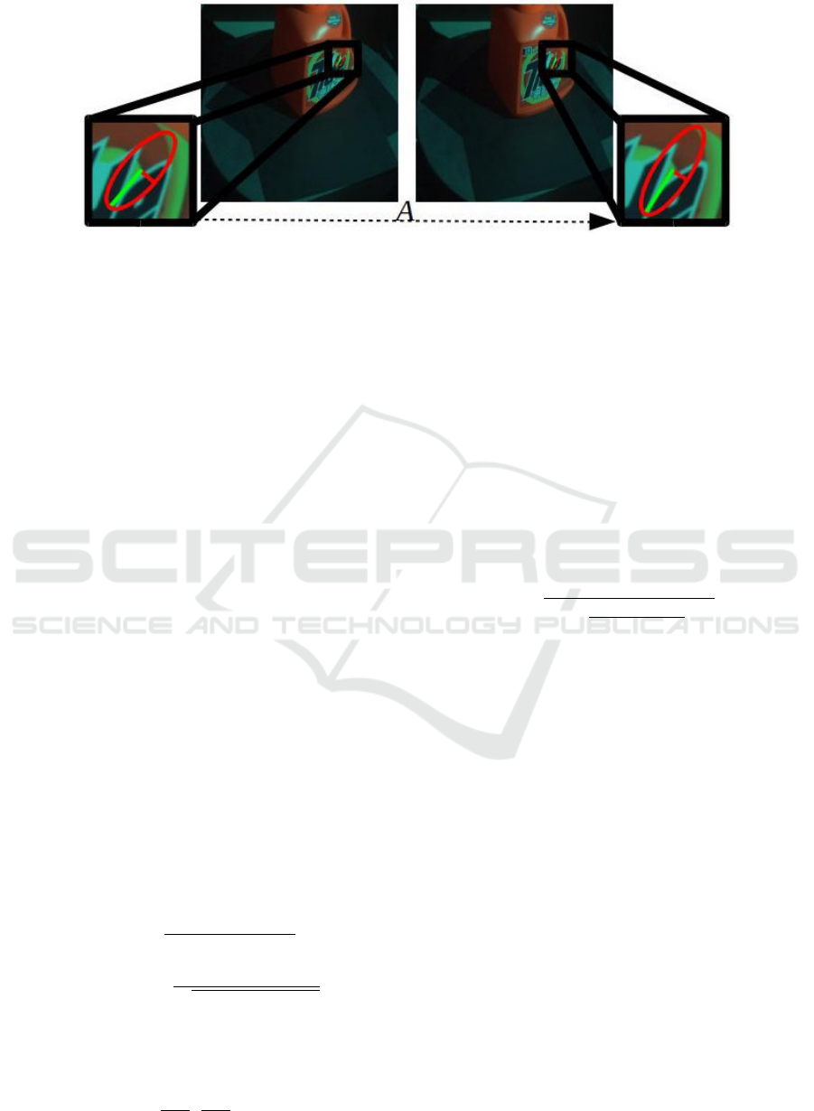
Figure 1: The afﬁne transformation (A) of corresponding features. The ellipses show the afﬁne shapes around the features. A

approximately transforms the local region of the ﬁrst image to that of the second one.

2. Estimate the afﬁne shape using M.

3. Normalize the afﬁne shape into a circle using

1/2

4. Detect new position and scale in the normalized

region.

5. Goto (2), if the the eigenvalues of M are not equal.

The iteration always converges, the obtained afﬁne

shape is described as an ellipse.

The scale and shape selections described above

can be applied to any point feature. Mikolajczyk also

proposed the Hessian-Laplace and Hessian-Afﬁne

detectors, which use the Hesse matrix for extracting

features, instead of the Harris. The matrix is as fol-

lows:

H(x) =



(x,σ

) f

(x,σ

)

(x,σ

) f

(x,σ

)



, (2)

where f

(x,σ

) is the second order Gaussian smoot-

hed image derivatives. The Hesse matrix can be used

to detect blob-like features.

Edge-based Regions (EBR). (Tuytelaars and

Van Gool, 2004) introduced a method to detect afﬁne

covariant regions around the corners. The Harris

corner detector is used along with standard Canny

edge detector. Afﬁne regions are found where two

edges meet at a corner. The corner point (p) and two

points moving along the two edges (p

and p

) deﬁne

a parallelogram. The ﬁnal shape is found, where the

region yields extremum in the following function:

f (Ω) = abs



|(p − p

)(q − p

|(p − p

)(p − p



− (M

)

(3)

where

Ω

(x,y)x

dx dy,





and p

is the center of gravity. The parallelogram re-

gions are then converted to ellipses.

Intensity-extrema-based Regions (IBR). While

EBR ﬁnd features at the corners and edges, IBR ex-

tracts afﬁne regions based on intensity properties.

First, the image is smoothed, then the local extrema

is selected using non-maximum suppression. These

points cannot be detected precisely, however they are

robust to monotonic intensity transformations. Rays

are cast from the local extremum to every direction,

and the following function is evaluated on each ray:

(t) =

abs(I(t) − I

)

max



abs(I(t)−I

)dt



(4)

where, t, I(t), I

and d are the arclength along the

ray, the intensity at position, the intensity extremum

and a small number to prevent dividing by 0, respecti-

vely. The function yields extremum where the inten-

sity suddenly changes. The points along the cast rays

deﬁne an usually irregularly-shaped region, which is

replaced by an ellipse having the same moments up to

the second order.

TBMR. Tree-Based Morse Regions is introduced

in (Xu et al., 2014). This detector is motivated by

Morse theory, selecting critical regions as features,

using the Min and Max-tree. TBMR can be seen as

a variant of MSER, however, TBMR is invariant to

illumination change and needs less number of para-

meters.

SURF. SURF is introduced in (Bay et al., 2008). It

is the fast approximation of SIFT (Lowe, 2004). The

Hessian matrix is roughly approximated using box ﬁl-

ters, instead of Gaussian ﬁlters. This makes the detec-

tor relatively fast comparing to the others. Despite the

approximations, SURF can ﬁnd reliable features.

VISAPP 2019 - 14th International Conference on Computer Vision Theory and Applications

706

3 GT DATA GENERATION

In order to quantitatively compare the detectors per-

formance and the reliability of afﬁne transformations,

ground truth (GT) data is needed. Many comparison

databases (Mikolajczyk et al., 2005; Cordes et al.,

2013; Zitnick and Ramnath, 2011) are based on ho-

mography, which is extracted from the observed pla-

nar object. Images are taken from different camera

positions, and the GT afﬁne transformations are cal-

culated from the homography. Instead of this, our

comparison is based on images captured by a quad-

copter in a real world environment and the GT afﬁne

transformation is extracted directly from constrained

movement of the quadcopter. This work is motivated

by the fact, that the afﬁne parameters can be calcula-

ted more precisely from the constrained movements,

than from the homography. Moreover, if the parame-

ters of the motion are estimated, the GT location of

the features can be determined as well. Thus, it is

possible to compare not only the afﬁne transformati-

ons, but the locations of the features, additionally. In

this section, these restricted movements, and the com-

putations of the corresponding afﬁne transformations

are introduced.

3.1 Rotation

In case of the rotation movement, the quadcopter

stays at the same position, and rotates around its verti-

cal axis. Thus, the translation vector of the movement

is equivalent to 0 all the time. The rotation matrices

between the images can be computed if the degrees

and center of the rotation are known. Example ima-

ges are given in Fig. 2. The ﬁrst row shows the images

taken by the quadcopter, and the second row shows

colored boxes, which are related by afﬁne transfor-

mations.

Let α

be the degree of rotation in radians, then the

rotation matrix is deﬁned as follows:



cosα

−sinα

sinα

cosα



. (5)

This matrix describes the transformation of corre-

sponding afﬁne shapes, in case of the rotation mo-

vement. Let us assume that corresponding feature

points in the images are given, then the relation of the

corresponding features can be expressed as follows:

= v +R



− v



, (6)

where p

, α

, v are the p-th feature location in the

f -th image, the degree of rotation between the ﬁrst

Testing data are submitted as supplementary material.

to the f -th image and the center of rotation, respecti-

vely. The latter one is considered constant during the

rotation movement.

To estimate the degree and center of the rotation,

the Euclidean distances of the selected and estimated

features have to be minimized. The cost function des-

cribing the error of estimation is as follows:

∑

f =2

∑

i=1



− R



− v



− v



, (7)

where F and P are the number of frames and selected

features, respectively. The minimization can be sol-

ved by an alternation algorithm. The alternation itself

consist of two steps: (i) estimation of the center of

rotation v and (ii) estimation of rotation angles α

3.1.1 Estimation of Rotation Center

The problem of rotation center estimation can be for-

malized as Av = b, where

A =







− I







,b =







− p







. (8)

The optimal solution in the lest-squares sense is given

by the pseudo-inverse of A:

v =





−1

b (9)

3.1.2 Estimation of Rotating Angles

The rotation angles are separately estimated for each

image. The estimation can be written in a linear form

Cx = d subject to x

x = 1, where



cosα

sinα



= d. (10)

The coefﬁcient matrix C and vector d are as follows:

C =







− u v − y

− v x

− u

− u v − y

− v x

− u







d =







− u

− v

− u

− v







, (11)

where

= p

and [u,v]

= v.

The optimal solution for this problem is given by

one of the roots of a four degree polynomial as it is

written in the appendix.

Convergence. The steps described above are repeated

one after the other, iteratively. The speed of conver-

gence does not matter for our application. However,

we empirically found that it convergences after a few

Quantitative Afﬁne Feature Detector Comparison based on Real-World Images Taken by a Quadcopter

707

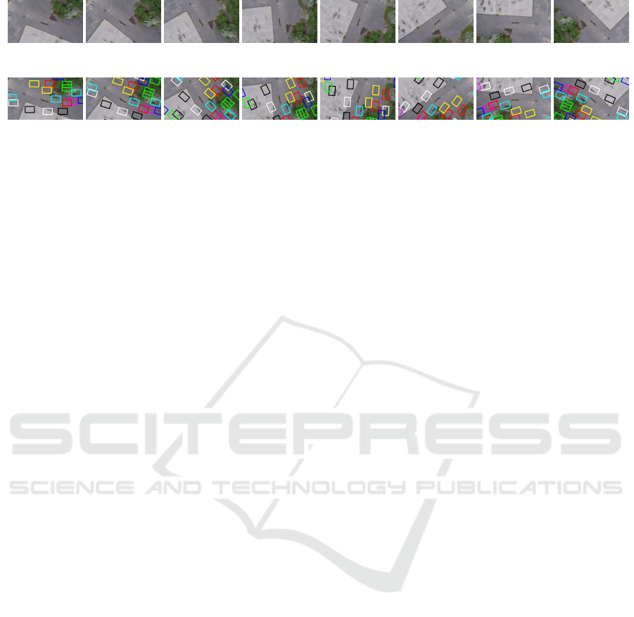
(a) Example images from the sequence.

(b) Colored boxes indicate corresponding areas computed by the rotation parameters. Images are the same as in the ﬁrst row.

Figure 2: Images are taken while the quadcopter is rotating around its vertical axis, while its position is ﬁxed.

iterations, when the center of the image is used as the

initial value for the center of the rotation.

Ground Truth Afﬁne Transformations. The afﬁne

transformations are easy to determine: they are equal

to the rotation: A = R.

3.2 Uniform Motion: Front View

For this test case, the quadcopter moves along a

straight line and does not rotate. Thus, the rotation

matrix relative to the camera movement is equal to the

identity. The camera faces to the front, thus the Focus

of Expansion (FOE) can be computed. The FOE is

the projection of the spatial line of movement at the

inﬁnity to the camera image. It is also an epipole in

the image, meaning that all epipolar lines intersect at

the FOE. The epipolar lines can be determined from

the projections of corresponding spatial points. Fig. 3

shows an example image sequence for this motion. In

the second row, the red dot indicates the calculated

FOE, and the blue lines mark the epipolar lines.

The maximum likelihood estimation of the FOE

can be solved by a numerical minimization of the sum

of squared orthogonal distances from the projected

points and the measured epipolar lines (Hartley and

Zisserman, 2003). Thus, the cost function to be mini-

mized contains the sum of all feature distance to the

related epipolar line. It can be formalized as follows:

∑

f =1

∑

i=1





− m





−sinβ

cosβ



, (12)

where m and β

are the FOE and the angle between

the epipolar line and the X axis. Note, that the ex-

pression [−sinβ

,cosβ

]

is the normal vector of the

i-th epipolar line. This cost function can be minimi-

zed with an alternation, iteratively reﬁning the FOE

and angles of epipolar lines. The center of the image

is used as the initial value for the FOE, then the epi-

polar lines can be calculated as it is described in the

following subsection.

3.2.1 Estimation of Epipolar Lines

The epipolar lines intersect at the FOE, because a

pure translation motion is considered. Moreover, the

epipolar lines connecting corresponding features with

the FOE are the same along the images. Each angle

between the epipolar lines and the horizontal (image)

axis can be computed as a homogeneous system of

equations Ax = 0 with constraint x

x = 1 as follows:

A =







− m

− x

− m

− x







,x =



cosβ

sinβ



, (13)

where [m

] = m and

= p

are the coor-

dinates of the FOE and that of the selected features,

respectively.

The solution which minimizes the cost function is

obtained as the eigenvector (v) of the smallest eigen-

value of matrix A

A. Then, β

= atan2(v

3.2.2 Estimation of the Focus of Expansion

The FOE is located where the epipolar lines of the

features intersect, thus the estimation of the FOE can

be formalized as a linear system of equations Am = b,

where

A =







−sinβ

cosβ

−sinβ

cosβ

−sinβ

cosβ

−sinβ

cosβ

−sinβ

cosβ







, (14)

VISAPP 2019 - 14th International Conference on Computer Vision Theory and Applications

708

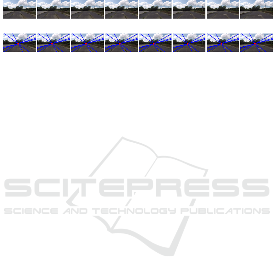
(a) A few images of the sequence.

(b) Red dot marks the FOE, blue lines are the epipolar ones. Images are the same as in the ﬁrst row.

Figure 3: The images are taken while the quadcopter is moving parallel to the ground.

and

b =







∗ cosβ

− x

sinβ

∗ cosβ

− x

sinβ

∗ cosβ

− x

sinβ

∗ cosβ

− x

sinβ

∗ cosβ

− x

sinβ







. (15)

This system of equations can be solved with the

Pseudo inverse of A. Thus v =





−1

Ab.

3.2.3 The Fundamental Matrix

The steps explained above are iteratively repeated

until convergence. The GT afﬁne transformation is

impossible to compute in an unknown environment,

because it depends on the surface normal (Barath

et al., 2015), and the normals are varying from fe-

ature to feature. However, some constraints can be

achieved if the fundamental matrix is known. The

fundamental matrix describes the transformation of

epipolar lines between stereo images in a static envi-

ronment. It is the composition of the camera matrices

and the parameters of camera motion as follows:

F = K

−T

R[t]

−1

, (16)

where K, R and [t]

are the camera matrix, rotation

matrix and the matrix representation of the cross pro-

duct, respectively. The fundamental matrix can be

computed as F = [v]

from the FOE if the relative mo-

tion of cameras contains only translation (Hartley and

Zisserman, 2003). If the fundamental matrix for two

images is known, the closest valid afﬁne transforma-

tion can be determined (Barath et al., 2016). These

closest ones are labelled as ground-truth transforma-

tions in our experiments. The details of the compa-

rison using the fundamental matrix can be found in

Sec. 4.2.

3.3 Uniform Motion: Bottom View

This motion is the same as described in the previous

section. However, the camera observes the ground,

instead of facing forward. Since the movement is pa-

rallel to the image plane, it can be considered as a de-

generative case of the previous one, because the FOE

is located at the inﬁnity. In this scenario the features

of the ground are related by a pure translation between

the images as the ground is planar. The projections

of the same corresponding features form a line in the

camera images, but these epipolar lines are parallel to

each other, and also parallel to the motion of the quad-

copter. Fig. 4 shows example images of this motion

and colored boxes related by the afﬁne transformati-

ons.

Let us denote the angle between the epipolar lines

and the X axis by γ, and l

denotes a point which lies

on the i-th epipolar line. The cost function to be mini-

mized contains the squared distances of the measured

points to the related epipolar lines:

∑

f =1

∑

i=1





− l





−sinγ

cosγ



. (17)

The alternation minimizes the error with reﬁning the

angle of the epipolar lines (γ) ﬁrst, then their points

). The ﬁrst part of the alternation can be written

as a homogeneous system of equations Ax = 0 with

respect to x

x = 1, similarly to Eq. 13, but it contains

all points for all images:







− l









−sinγ

cosγ



= 0, (18)

the solution is obtained as the eigenvector of the smal-

lest eigenvalue of matrix A

A, then γ = atan2(v

The second step of the alternation reﬁnes the

points located on the epipolar lines. The equation can

Quantitative Afﬁne Feature Detector Comparison based on Real-World Images Taken by a Quadcopter

709

(a) Example images for uniform motion, bottom view.

(b) The colored boxes indicates the same areas computed by the motion parameters.

Figure 4: The images are taken while the quadcopter is moving forward.

be formed as Ax = b, where







cosγ sinγ

















cosγ + y

sinγ

cosγ + y

sinγ







(19)

the point on the line is given by the pseudoinverse of

A, l =





−1

Ab.

Ground Truth Afﬁne Transformations The GT

afﬁne transformations for forward motion with a

bottom-view camera is a simple identity:

A = I (20)

3.4 Scaling

This motion is generated by the sinking of the quad-

copter, while the camera observes the ground. The

direction of the motion is approximately perpendicu-

lar to the camera plane, thus this can be considered

as a special case of the Uniform Motion: Front View.

The only difference is that the ground can be conside-

red as a plane, thus the parameters of the motion and

the afﬁne transformation can be precisely calculated.

Fig. 5 ﬁrst row shows an example images captured

during the motion.

Because of the direction of the movement and the

camera plane are not perpendicular, the FOE and the

epipolar lines for the corresponding selected features

can be computed. It is also true, that during the sin-

king of the quadcopter, the features move along their

corresponding epipolar line. See Seq. 3.2 for the com-

putation of the FOE and epipolar lines.

The corresponding features are related in the ima-

ges by the parameter of the scaling. Let s be the sca-

ling parameter, then the distances between the featu-

res and the FOE are related by s. This can be forma-

lized as follows:



− v



= s



− v



i ∈ [1,P]. (21)

Thus, the parameter of the scale is given, by the

average of the fraction of the distances:

∑

i=1



− v



− v



. (22)

Ground Truth Afﬁne Transformations. The GT af-

ﬁne transformations for the scaling is trivially a sim-

ple scaled identity:

= sI (23)

4 EVALUATION METHOD

The evaluation of the feature detectors is twofold. In

the ﬁrst comparison, the detection of features location

and afﬁne parameters are evaluated. To compare the

feature locations and afﬁne parameters, the camera

motion needs to be known. These can be calculated

for each motion described in the previous section, ho-

wever, for the Uniform Motion: Front View, it is not

possible. Thus, a second comparison is carried out,

which uses only the fundamental matrix instead of the

motion parameters.

4.1 Afﬁne Evaluation

Location error. The location of the GT feature can

be determined by the location of the same feature in

the previous image, and the parameters of the motion.

The calculation of the motion parameter differs from

motion to motion, the details can be found in the re-

lated sections. The error of the feature detection is

the Euclidean distance of the GT and the estimated

feature:

Err

det

estimated

) =

estimated

− P

, (24)

where P

, P

estimated

are the GT and estimated feature

points, respectively.

Afﬁne Error. While the error of the feature detection

is based on the Euclidean distance, the error of afﬁne

transformation is calculated using the Frobenius norm

of the difference matrix of the estimated and GT afﬁne

transformation. It can be formalized as follows:

Err

a f f

estimated

) =

estimated

− A

(25)

where A

estimated

are the GT and estimated afﬁne

transformations, respectively. The Frobenius norm

VISAPP 2019 - 14th International Conference on Computer Vision Theory and Applications

710

(a) Example images for the scaling test.

(b) The colored boxes indicate the same areas computed by the scaling parameters.

Figure 5: The images are taken while the quadcopter is sinking.

is chosen, because it has a geometrical meaning of

the related afﬁne transformations, see (Barath et al.,

2016) for details.

4.2 Fundamental Matrix Evaluation

For the motion named as Uniform Motion: Front

View, the afﬁne transformations and parameters of

the motion can not be estimated. The objects, which

are closer to the camera move more pixels between

the successive images, than objects located at the dis-

tance. Only the direction of the moving features can

be calculated. That is the epipolar line that goes

through the feature and the FOE. However, the funda-

mental matrix can be precisely calculated from FOE,

F = [v]

and it can be used to reﬁne the afﬁne trans-

formations.

The reﬁned afﬁne transformations are considered

as GT, and used for the calculation of afﬁne errors, as

it is described in the previous section. (Barath et al.,

2016) introduced the algorithm to ﬁnd the closest af-

ﬁne transformations corresponding to the fundamen-

tal matrix. The paper states that it can be determi-

ned by solving a six-dimensional linear problem if the

Lagrange-multiplier technique is applied for the con-

straints for the fundamental matrix.

For quantifying the quality of an afﬁne transfor-

mation, the closest valid afﬁne transformation is com-

puted ﬁrst by the method of (Barath et al., 2016).

Then the difference matrix between the original and

closest valid afﬁne transformation is computed. The

quality is given by the Frobenius norm of this diffe-

rence matrix.

5 COMPARISON

Eleven afﬁne feature detectors have been compared in

our tests. The implementations are downloaded from

the website of Visual Geometry Group, University of

Oxford

, except the TBMR, which is available on the

www.robots.ox.ac.uk/ vgg/research/afﬁne/index.html

website of the author

. Most of the methods are intro-

duced in Sec. 2. Additionally to those, HARHES and

SEDGELAP are added to the comparison. HARHES

is the composition of HARAFF and HESAFF, while

SEDGELAP ﬁnds shapes along the edges, using the

Laplace operator.

After the features are extracted from the images,

feature matching is done considering SIFT descrip-

tors. The ratio test published in (Lowe, 2004) was

used for outlier ﬁltering. Finally, the afﬁne transfor-

mations are calculated for the ﬁltered matches. The

detectors determine only the elliptical area of the af-

ﬁne shapes, without orientation. The orientation is

assigned to the areas using the SIFT descriptor in a

separate step. Finally, the afﬁne transformation of the

matched feature is given by:

A = A

)

−1

, (26)

where A

i ∈ [1, 2] are the local afﬁne areas deﬁned

by ellipses, and the related rotation matrices assigned

by the SIFT descriptor, respectively.

Table 1 summarizes the number of features, num-

ber of matched features and running time of the de-

tectors on the tests. SEDGELAP and HARHES ﬁnd

the most features, however, the high number of fea-

tures makes the matching more complicated and time

consuming. In general, EBR, IBR and MSER ﬁnd

hundreds of features, the Harris based methods (HA-

RAFF, HARLAP) ﬁnd approximately ten to twenty

thousand, and the Hessian based methods (HESAFF,

HESLAP) ﬁnd a few thousands of features. The ra-

tio test (Lowe, 2004), used for outlier ﬁltering, exclu-

des some feature matches. The second row of each

test sequence in Table 1 shows the number of fea-

tures after matching and outlier ﬁltering. Note, that

approximately 50% of features are lost due to the ra-

tio test. The running time of the methods are shown

in the third rows of each test sequence. These ti-

mes highly depend on the image resolution, which is

5MP in our tests. Each implementation was run on

the CPU, using one core of the machine. Obviously,

MSER is the fastest method, followed by SURF and

http://laurentnajman.org/index.php?page=tbmr

Quantitative Afﬁne Feature Detector Comparison based on Real-World Images Taken by a Quadcopter

711

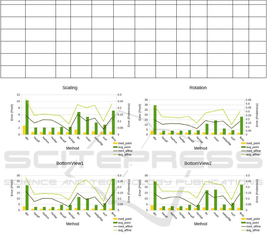
Table 1: Number of features, number of matched features and required running time for test sequences. The columns are the

methods and the rows (triplets) are the test sequences. First row of each sequence shows the number of detected features.

The number of matched features are shown in the second row. The third row of each test sequence contains the required

running times.

EBR HARAFF HARHES HARLAP HESAFF HESLAP IBR MSER SEDGELAP SURF TBMR

Scaling

# All 217 18720 21198 19033 3866 3994 1277 336 20132 783 4122

# Matched 91 8369 9544 8534 1702 1757 678 235 10071 636 2259

Running time (s) 20.43 3.27 2.32 2.06 1.19 0.97 7.59 0.41 3.29 0.65 0.68

Rotation

# All 114 12686 14266 12795 2655 2751 892 223 13173 508 3141

# Matched 33 5235 5943 5294 1070 1111 395 133 5872 390 1447

Running time (s) 18.01 2.21 1.69 1.56 0.91 0.77 6.27 0.35 2.41 0.54 0.54

Bottonview1

# All 59 7514 8122 7629 1211 1216 441 92 7222 204 2688

# Matched 27 3450 3730 3503 522 524 226 64 3743 169 1049

Running time (s) 18.09 1.69 1.37 1.30 0.80 0.73 5.52 0.38 1.85 0.51 0.67

Bottonview2

# All 26 12484 13020 12615 1119 1135 588 117 9461 139 3051

# Matched 8 4451 4681 4506 418 426 241 68 4094 107 1037

Running time (s) 20.49 2.22 1.65 1.64 0.78 0.72 5.25 0.36 2.11 0.57 0.95

FrontView1

# All 78 10128 13639 10415 4708 5032 695 233 14869 803 2083

# Matched 36 4623 6476 4758 2444 2583 416 164 7650 653 1058

Running time (s) 17.97 3.16 2.12 1.66 1.70 1.19 8.47 0.29 2.67 0.81 0.76

FrontView2

# All 59 9210 11193 9369 2108 2812 592 50 12345 511 1856

# Matched 30 4615 5764 4703 1192 1617 398 38 7275 447 1034

Running time (s) 15.56 2.07 1.65 1.48 1.01 0.87 6.58 0.29 2.31 0.65 0.55

Figure 6: The error of afﬁne evaluation. The error of feature detection is measured in pixels, and can be seen on the left axis.

The error of afﬁne transformations is given by the Frobenius norm, it is plotted on the right axis. The average and median

values for both the afﬁne and detection errors are shown.

TBMR. The Hessian based methods need approxima-

tely 1 second to process an image, while Harris based

methods need 1.5 or 2 more times. The slowest are

IBR and EBR. Note that, by parallelism and/or GPU

implementations, the running times may show diffe-

rent results.

5.1 Afﬁne Evaluation

The ﬁrst evaluation uses the estimated camera moti-

ons and afﬁne transformation introduced in Sec. 3.

The quantitative evaluation is twofold, since the lo-

calization of features and accuracy of afﬁne transfor-

mation can both be evaluated.

Four test sequences are captured. One for the sca-

ling, one for the rotation and two for the Uniform Mo-

tion: Bottom View motions. See Fig. 2 for the rota-

tion, Fig. 5 for the scale, ﬁrst row of Fig. 4 and Fig. 7

for the Uniform Motion: Bottom View test images.

Fig. 6 summarizes the errors for the detectors. The

average and median error of feature detection can be

seen on the bar-charts, where the left vertical axis

mark the Euclidean distance between the estimated

and GT feature, measured in pixels. The average and

median error of the afﬁne transformations are visuali-

zed as green and black lines, respectively. The mea-

VISAPP 2019 - 14th International Conference on Computer Vision Theory and Applications

712

(a) Example images for the BottonView2 test.

(b) Example images for the FrontView test.

Figure 7: The images are taken while the quadcopter is moving parallel to the ground. First Row: The camera observes the

ground. Second row: It faces to the front.

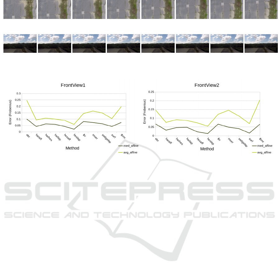
Figure 8: The error of Fundamental Matrix Evaluation.

sure is given by the Frobenius norm of the difference

of the GT and estimated afﬁne transformations. The

quantity of the error can be seen at the right vertical

axis of the charts.

The charts of Fig. 6 indicate similar results for

the test sequences. The detection error is always the

lowest for the Hessian and Harris based methods in

average, indicating that these methods can ﬁnd featu-

res more accurately than others. This measure is the

highest for the EBR, IBR, MSER and TBMR. The

averages can even be higher than 10 pixels, except for

the scaling test case. Remark that the median values

are always lower than the averages, because despite of

the outlier ﬁltering, the false matches can yield large

detection error, which distorts the averages. Surpri-

singly, the afﬁne error of HESLAP and SURF is the

lowest, while that of the EBR, IBR and TBMR is the

highest in all test cases.

5.2 Fundamental Matrix Evaluation

In case of the fundamental matrix evaluation, the

quadcopter moves forward, perpendicular to the

image plane. Objects are located at different distan-

ces from the camera, thus the GT afﬁne transforma-

tion and GT position of features can not be recovered.

In this comparison, the fundamental matrix is used to

reﬁne the estimated afﬁne transformations. Then, the

error is measured by Frobenius norm of the difference

matrix of the estimated and reﬁned afﬁne transforma-

tion.

Two test scenarios are considered. The example

images of the ﬁrst one can be seen in Fig. 3, where the

height of the quadcopter was approximately 2 meters.

The images of the second scenario are shown in the

second row of Fig. 7, these images are taken at around

the top of the trees.

Fig. 8 shows the error of the afﬁne transformati-

ons. Two test sequences are captured, each shows

similar result. The HARAFF, HARLAP and SURF

afﬁne transformation yield the least afﬁne errors. The

characteristic of the errors is similar to that in the pre-

vious comparison.

6 CONCLUSIONS

We have compared the most popular afﬁne matcher

algorithms in this paper. The main novelty of our

study is that the comparisons have been carried out

on realistic images taken by a quadcopter. Our test

sequences consists of more complex test cases than a

simple homography estimation: rotation and scaling

appear in the test as well. As a side effect, point ma-

tchers has also been compared as afﬁne matching is

impossible without point matching.

The most important conclusion of the tests that the

performance of the afﬁne detectors do not depend on

the type of the sequence. Based on the results, the

authors of this paper suggest to apply Harris-based,

Quantitative Afﬁne Feature Detector Comparison based on Real-World Images Taken by a Quadcopter

713

Hessian-based and SURF algorithm to retrieve high

quality afﬁne transformations from image pairs.

ACKNOWLEDGEMENTS

EFOP-3.6.3-VEKOP-16-2017-00001: Talent Mana-

gement in Autonomous Vehicle Control Technologies

– The Project is supported by the Hungarian Govern-

ment and co-ﬁnanced by the European Social Fund.

REFERENCES

Alcantarilla, P. F., Bartoli, A., and Davison, A. J. (2012).

Kaze features. In Fitzgibbon, A., Lazebnik, S., Pe-

rona, P., Sato, Y., and Schmid, C., editors, Computer

Vision – ECCV 2012, pages 214–227, Berlin, Heidel-

berg. Springer Berlin Heidelberg.

Barath, D., Matas, J., and Hajder, L. (2016). Accurate

closed-form estimation of local afﬁne transformati-

ons consistent with the epipolar geometry. In Procee-

dings of the British Machine Vision Conference 2016,

BMVC 2016, York, UK, September 19-22, 2016.

Barath, D., Moln

ar, J., and Hajder, L. (2015). Optimal sur-

face normal from afﬁne transformation. In VISAPP

2015 - Proceedings of the 10th International Confe-

rence on Computer Vision Theory and Applications,

Volume 3, Berlin, Germany, 11-14 March, 2015., pa-

ges 305–316.

Bay, H., Ess, A., Tuytelaars, T., and Van Gool, L. (2008).

Speeded-up robust features (surf). Comput. Vis. Image

Underst., 110(3):346–359.

Cordes, K., Rosenhahn, B., and Ostermann, J. (2013).

High-resolution feature evaluation benchmark. In

Wilson, R., Hancock, E., Bors, A., and Smith, W., edi-

tors, Computer Analysis of Images and Patterns, pages

327–334, Berlin, Heidelberg. Springer Berlin Heidel-

berg.

Harris, C. and Stephens, M. (1988). A combined corner

and edge detector. In In Proc. of Fourth Alvey Vision

Conference, pages 147–151.

Hartley, R. and Zisserman, A. (2003). Multiple View Ge-

ometry in Computer Vision. Cambridge University

Press, New York, NY, USA, 2 edition.

Leutenegger, S., Chli, M., and Siegwart, R. Y. (2011).

Brisk: Binary robust invariant scalable keypoints. In

Proceedings of the 2011 International Conference on

Computer Vision, ICCV ’11, pages 2548–2555, Wa-

shington, DC, USA. IEEE Computer Society.

Lowe, D. G. (2004). Distinctive image features from scale-

invariant keypoints. Int. J. Comput. Vision, 60(2):91–

110.

Mikolajczyk, K. and Schmid, C. (2002). An afﬁne invariant

interest point detector. In Heyden, A., Sparr, G., Niel-

sen, M., and Johansen, P., editors, Computer Vision

— ECCV 2002, pages 128–142, Berlin, Heidelberg.

Springer Berlin Heidelberg.

Mikolajczyk, K., Tuytelaars, T., Schmid, C., Zisserman, A.,

Matas, J., Schaffalitzky, F., Kadir, T., and Gool, L. V.

(2005). A comparison of afﬁne region detectors. In-

ternational Journal of Computer Vision, 65(1):43–72.

Pusztai, Z. and Hajder, L. (2017). Quantitative comparison

of afﬁne invariant feature matching. In Proceedings of

the 12th International Joint Conference on Computer

Vision, Imaging and Computer Graphics Theory and

Applications (VISIGRAPP 2017) - Volume 6: VISAPP,

Porto, Portugal, February 27 - March 1, 2017., pages

515–522.

Shi, J. and Tomasi, C. (1994). Good features to track.

Tareen, S. A. K. and Saleem, Z. (2018). A comparative

analysis of sift, surf, kaze, akaze, orb, and brisk. In

International Conference on Computing, Mathematics

and Engineering Technologies (iCoMET).

Tuytelaars, T. and Mikolajczyk, K. (2008). Local invariant

feature detectors: A survey. Found. Trends. Comput.

Graph. Vis., 3(3):177–280.

Tuytelaars, T. and Van Gool, L. (2004). Matching widely

separated views based on afﬁne invariant regions. In-

ternational Journal of Computer Vision, 59(1):61–85.

Xu, Y., Monasse, P., Graud, T., and Najman, L. (2014).

Tree-based morse regions: A topological approach to

local feature detection. IEEE Transactions on Image

Processing, 23(12):5612–5625.

Zitnick, L. and Ramnath, K. (2011). Edge foci interest

points. International Conference on Computer Vision.

APPENDIX

The goal is to show how the following equation:

Ax = b

can be solved subject to x

x = 1. The cost function

must be written with the so-called Lagrangian multi-

plier λ. It is as follows:

J = (Ax − b)

(Ax − b) + λx

The optimal solution is given by the derivative of the

cost function w.r.t x.

∂J

∂x

= 2A

(Ax − b) + 2λx = 0.

Therefore the optimal solution is as follows:

x = (A

A + λI)

−1

For the sake of simplicity, we introduce the vector v =

b and the symmetric matrix C = A

A, then:

x = (C + λI)

−1

Finally, the constraint x

x = 1 has to be considered:

(C + λI)

−T

(C + λI)

−1

v = 1.

By deﬁnition, it can be written that:

(C + λI)

−1

ad j(C + λI)

det(C + λI)

VISAPP 2019 - 14th International Conference on Computer Vision Theory and Applications

714

C =





then

C + λI =



+ λ c

+ λ



The determinant and adjoint matrix of C + λI can be

written as:

det(C + λI) = (c

+ λ)(c

+ λ) − c

and

ad j(C + λI) =



+ λ −c

−c

+ λ





+ λ −c

−c

+ λ







λ + c

− c

λ + c

− c



Furthermore, the expression v

(C + λI)

−T

(C +

λI)

−1

v = 1 can be rewritten as

ad j

(C + λI)ad j(C + λI)

det(C + λI)det(C + λI)

v = 1,

ad j

(C + λI)ad j(C + λI)v = det

(C + λI).

Both sides of the equation contain polynomials.

The degrees of the left and right sides are 2n − 2 and

2n, respectively. If the expression in the sides are

subtracted by each other, a polynomial of degree 2n

is obtained. Note that, n = 2 in the discussed case,

i.e planar motion. The optimal solution is obtained

as the real roots of this polynomial. The vector cor-

responding to the estimated λ

, i ∈ 1, 2, is calculated

as g

= (L + λ

−1

r. Then the vector with minimal

norm

− h

is selected as the optimal solution of

the problem.

Quantitative Afﬁne Feature Detector Comparison based on Real-World Images Taken by a Quadcopter

715