Semantic Image Inpainting through Improved Wasserstein Generative

Adversarial Networks

Patricia Vitoria

, Joan Sintes

and Coloma Ballester

Department of Information and Communication Technologies, University Pompeu Fabra, Barcelona, Spain

Keywords:

Generative Models, Wasserstein GAN, Image Inpainting, Semantic Understanding.

Abstract:

Image inpainting is the task of ﬁlling-in missing regions of a damaged or incomplete image. In this work

we tackle this problem not only by using the available visual data but also by incorporating image semantics

through the use of generative models. Our contribution is twofold: First, we learn a data latent space by

training an improved version of the Wasserstein generative adversarial network, for which we incorporate a

new generator and discriminator architecture. Second, the learned semantic information is combined with

a new optimization loss for inpainting whose minimization infers the missing content conditioned by the

available data. It takes into account powerful contextual and perceptual content inherent in the image itself.

The beneﬁts include the ability to recover large regions by accumulating semantic information even it is

not fully present in the damaged image. Experiments show that the presented method obtains qualitative

and quantitative top-tier results in different experimental situations and also achieves accurate photo-realism

comparable to state-of-the-art works.

1 INTRODUCTION

The goal of image inpainting methods is to recover

missing information of occluded, missing or corrup-

ted areas of an image in a realistic way, in the sense

that the resulting image appears as of a real scene. Its

applications are numerous and range from the auto-

matization of cinema post-production tasks enabling,

e.g., the deletion of annoying objects, to new view

synthesis generation for, e.g., broadcasting of sport

events. Interestingly, it is a pervasive and easy task

for a human to infer hidden areas of an image. Given

an incomplete image, our brain unconsciously recon-

structs the captured real scene by completing the gaps

(called holes or inpainting masks in the inpainting li-

terature). On the one hand, it is acknowledged that lo-

cal geometric processes and global ones (such as the

ones associated to geometry-oriented and exemplar-

based models, respectively) are leveraged in the hu-

mans’ completion phenomenon. On the other hand,

humans use the experience and previous knowledge

of the surrounding world to infer from memory what

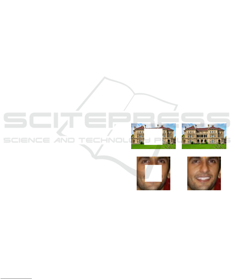
ﬁts the context of a missing area. Figure 1 displays

two examples of it; looking at the image in Figure

1(a), our experience indicates that one or more cen-

These two authors contributed equally

(a) (b)

Figure 1: Qualitative illustration of the task. Given the visi-

ble content in (a), our experience indicates that one or more

central doors would be expected in such incomplete buil-

ding. Thus, a plausible completion would be the one of (b).

Also, our brain automatically completes the image in (c)

with a face such as (d).

tral doors would be expected in such an incomplete

building and, thus, a plausible completion would be

the one of (b). Also, our trained brain automatically

completes Figure 1(c) with the missing parts of a face

such as the one shown in (d).

Mostly due to its inherent ambiguity and to the

complexity of natural images, the inpainting problem

remains theoretically and computationally challen-

Vitoria, P., Sintes, J. and Ballester, C.

Semantic Image Inpainting through Improved Wasserstein Generative Adversarial Networks.

DOI: 10.5220/0007367902490260

In Proceedings of the 14th International Joint Conference on Computer Vision, Imaging and Computer Graphics Theory and Applications (VISIGRAPP 2019), pages 249-260

ISBN: 978-989-758-354-4

249

ging, specially if large regions are missing. Classi-

cal methods use redundancy of the incomplete input

image: smoothness priors in the case of geometry-

oriented approaches and self-similarity principles in

the non-local or exemplar-based ones. Instead, using

the terminology of (Pathak et al., 2016; Yeh et al.,

2017), semantic inpainting refers to the task of infer-

ring arbitrary large missing regions in images based

on image semantics. Applications such as the identi-

ﬁcation of different objects which were jointly occlu-

ded in the captured scene, 2D to 3D conversion, or

image editing (in order to, e.g., removing or adding

objects and changing the object category) could be-

neﬁt from accurate semantic inpainting methods. Our

work ﬁts in this context. We capitalize on the under-

standing of more abstract and high level information

that unsupervised learning strategies may provide.

Generative methods that produce novel samples

from high-dimensional data distributions, such as

images, are ﬁnding widespread use, for instance in

image-to-image translation (Zhu et al., 2017a; Liu

et al., 2017), image synthesis and semantic manipu-

lation (Wang et al., ), to mention but a few. Currently

the most prominent approaches include autoregres-

sive models (van den Oord et al., ), variational au-

toencoders (VAE) (Kingma and Welling, 2013), and

generative adversarial networks (Goodfellow et al.,

2014). Generative Adversarial Networks (GANs) are

often credited for producing less burry outputs when

used for image generation. It consists of a framework

for training generative parametric models based on

a game between two networks: a generator network

that produces synthetic data from a noise source and a

discriminator network that differentiates between the

output of the genererator and true data. The approach

has been shown to produce high quality images and

even videos (Zhu et al., 2017b; Pumarola et al., 2018;

Chan et al., 2018).

We present a new method for semantic image in-

painting with an improved version of the Wasserstein

GAN (Arjovsky et al., 2017) including a new gene-

rator and discriminator architectures and a novel op-

timization loss in the context of semantic inpainting

that outperforms related approaches. More precisely,

our contributions are summarized as follows:

• We propose several improvements to the architec-

ture based on an improved WGAN such as the in-

troduction of the residual learning framework in

both the generator and discriminator, the removal

of the fully connected layers on top of convoluti-

onal features and the replacement of the widely

used batch normalization by a layer normaliza-

tion. These improvements ease the training of the

networks making them to be deeper and stable.

(a)

(b)

(c)

(d)

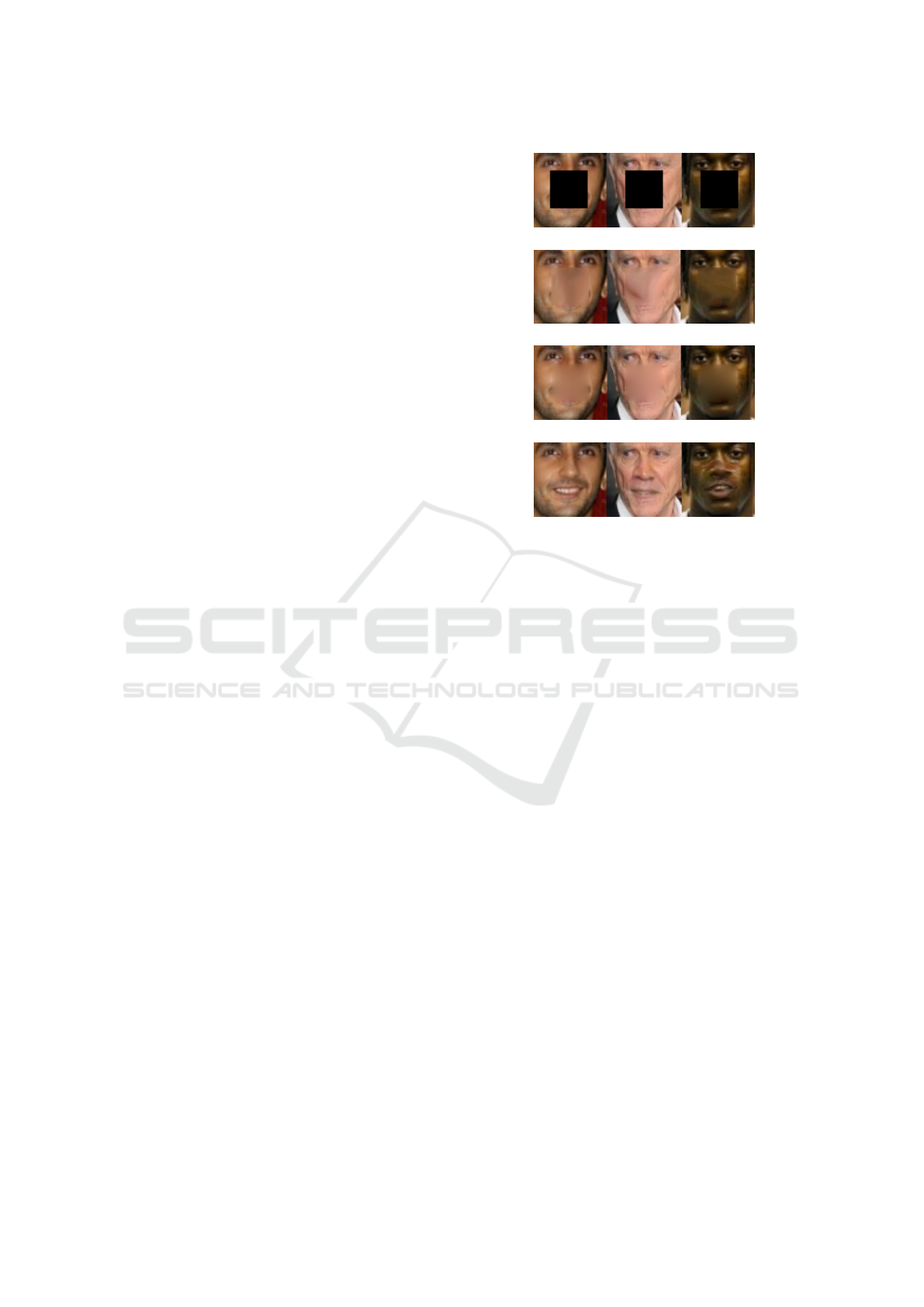
Figure 2: Image inpainting results using three different ap-

proaches. (a) Input images, each with a big hole or mask.

(b) Results obtained with the non-local method (Fedorov

et al., 2015). (c) Results with the local method (Getreuer,

2012). (d) Our semantic inpainting method.

• We deﬁne a new optimization loss that takes into

account, on the one side, the semantic information

inherent in the image, and, on the other side, con-

textual information that capitalizes on the image

values and gradients.

• We quantitatively and qualitatively show that our

proposal achieves top-tier results on two datasets:

CelebA and Street View House Numbers.

The remainder of the paper is organized as follows. In

Section 2, we review the related state-of-the-art work

focusing ﬁrst on generative adversarial networks and

then on inpainting methods. Section 3 details our

whole method. In Section 4, we present both quan-

titative and qualitative assessments of all parts of the

proposed method. Section 5 concludes the paper.

2 RELATED WORK

Generative Adversarial Networks. GAN learning

strategy (Goodfellow et al., 2014) is based on a game

theory scenario between two networks, the genera-

tor’s network and the discriminator’s network, having

adversarial objectives. The generator maps a source

of noise from the latent space to the input space and

the discriminator receives either a generated or a real

VISAPP 2019 - 14th International Conference on Computer Vision Theory and Applications

250

image and must distinguish between both. The goal

of this training procedure is to learn the parameters

of the generator so that its probability distribution is

as closer as possible to the one of the real data. To

do so, the discriminator D is trained to maximize the

probability of assigning the correct label to both real

examples and samples from the generator G, while

G is trained to fool the discriminator and to minimize

log(1−D(G(z))) by generating realistic examples. In

other words, D and G play the following min-max

game with value function V (G, D) deﬁned as follows:

min

max

V (D, G) =

x∼P

data

(x)

[logD(x)]

z∼p

(z)

[log(1 − D(G(z)))]

(1)

The authors of (Radford et al., 2015) introduced con-

volutional layers to the GANs architecture, and pro-

posed the so-called Deep Convolutional Generative

Adversarial Network (DCGAN). GANs have been

applied with success to many speciﬁc tasks such as

image colorization (Cao, 2017), text to image synthe-

sis (Reed et al., 2016), super-resolution (Ledig et al.,

2017), image inpainting (Yeh et al., 2017; Burlin

et al., 2017; Demir and

Unal, 2018), and image gene-

ration (Radford et al., 2015; Mao et al., 2017; Gulra-

jani et al., 2017; Nguyen et al., 2016), to name a few.

However, three difﬁculties still persist as challenges.

One of them is the quality of the generated images and

the remaining two are related to the well-known insta-

bility problem in the training procedure. Indeed, two

problems can appear: vanishing gradients and mode

collapse.

Vanishing gradients are specially problematic

when comparing probability distributions with non-

overlapping supports. If the discriminator is able to

perfectly distinguish between real and generated ima-

ges, it reaches its optimum and thus the generator

no longer improves the generated data. On the other

hand, mode collapse happens when the generator only

encapsulates the major nodes of the real distribution,

and not the entire distribution. As a consequence, the

generator keeps producing similar outputs to fool the

discriminator.

Aiming a stable training of GANs, several aut-

hors have promoted the use of the Wasserstein GAN

(WGAN). WGAN minimizes an approximation of the

Earth-Mover (EM) distance or Wasserstein-1 metric

between two probability distributions. The EM dis-

tance intuitively provides a measure of how much

mass needs to be transported to transform one dis-

tribution into the other distribution. The authors of

(Arjovsky et al., 2017) analyzed the properties of this

distance. They showed that one of the main bene-

ﬁts of the Wasserstein distance is that it is continuous.

This property allows to robustly learn a probability

distribution by smoothly modifying the parameters

through gradient descend. Moreover, the Wasserstein

or EM distance is known to be a powerful tool to com-

pare probability distributions with non-overlapping

supports, in contrast to other distances such as the

Kullback-Leibler divergence and the Jensen-Shannon

divergence (used in the DCGAN and other GAN ap-

proaches) which produce the vanishing gradients pro-

blem, as mentioned above. Using the Kantorovich-

Rubinstein duality, the Wasserstein distance between

two distributions, say a real distribution P

real

and an

estimated distribution P

, can be computed as

W (P

real

, P

) = supE

x∼P

real

[ f (x)] − E

x∼P

[ f (x)] (2)

where the supremum is taken over all the 1-Lipschitz

functions f (notice that, if f is differentiable, it im-

plies that k∇ f k ≤ 1). Let us notice that f in Equation

(2) can be thought to take the role of the discriminator

D in the GAN terminology. In (Arjovsky et al., 2017),

the Wasserstein GAN is deﬁned as the network whose

parameters are learned through optimization of

min

max

D∈D

x∼P

real

[D(x)] − E

x∼P

[D(x)] (3)

where D denotes the set of 1-Lipschitz functions. Un-

der an optimal discriminator (called a critic in (Ar-

jovsky et al., 2017)), minimizing the value function

with respect to the generator parameters minimizes

W (P

real

, P

). To enforce the Lipschitz constraint, the

authors proposed to use an appropriate weight clip-

ping. The resulting WGAN solves the vanishing pro-

blem, but several authors (Gulrajani et al., 2017; Ad-

ler and Lunz, 2018) have noticed that weight clip-

ping is not the best solution to enforce the Lipschitz

constraint and it causes optimization difﬁculties. For

instance, the WGAN discriminator ends up learning

an extremely simple function and not the real dis-

tribution. Also, the clipping threshold must be pro-

perly adjusted. Since a differentiable function is 1-

Lipschitz if it has gradient with norm at most 1 every-

where, (Gulrajani et al., 2017) proposed an alternative

to weight clipping: To add a gradient penalty term

constraining the L

norm of the gradient while opti-

mizing the original WGAN during training.

Recently, the Banach Wasserstein GAN (BW-

GAN) (Adler and Lunz, 2018) has been proposed ex-

tending WGAN implemented via a gradient penalty

term to any separable complete normed space. In this

work we leverage the mentioned WGAN (Gulrajani

et al., 2017) improved with a new design of the gene-

rator and discriminator architectures.

Image Inpainting. Most inpainting methods found

in the literature can be classiﬁed into two groups:

Semantic Image Inpainting through Improved Wasserstein Generative Adversarial Networks

251

model-based approaches and deep learning approa-

ches. In the former, two main groups can be dis-

tinguished: local and non-local methods. In local

methods, also denoted as geometry-oriented methods,

images are modeled as functions with some degree

of smoothness. (Masnou and Morel, 1998; Chan and

Shen, 2001; Ballester et al., 2001; Getreuer, 2012;

Cao et al., 2011). These methods show good perfor-

mance in propagating smooth level lines or gradients,

but fail in the presence of texture or for large missing

regions. Non-local methods (also called exemplar-

or patch-based) exploit the self-similarity prior by

directly sampling the desired texture to perform the

synthesis (Efros and Leung, 1999; Demanet et al.,

2003; Criminisi et al., 2004; Wang, 2008; Kawai

et al., 2009; Aujol et al., 2010; Arias et al., ; Hu-

ang et al., 2014; Fedorov et al., 2016). They provide

impressive results in inpainting textures and repeti-

tive structures even in the case of large holes. Howe-

ver, both type of methods use redundancy of the in-

complete input image: smoothness priors in the case

of geometry-based and self-similarity principles in

the non-local or patch-based ones. Figures 2(b) and

is shown in (a)) using a local method (in particular

(Getreuer, 2012)) and the non-local method (Fedorov

et al., 2015), respectively. As expected, the use of

image semantics improve the results, as shown in (d).

Current state-of-the-art is based on deep learning

approaches (Yeh et al., 2017; Demir and

Unal, 2018;

Pathak et al., 2016; Yang et al., 2017; Yu et al., ). (Pat-

hak et al., 2016) modiﬁes the original GAN architec-

ture by inputting the image context instead of random

noise to predict the missing patch. They proposed

an encoder-decoder network using the combination of

the L

loss and the adversarial loss and applied adver-

sarial training to learn features while regressing the

missing part of the image. (Yeh et al., 2017) propo-

ses a method for semantic image inpainting, which

generates the missing content by conditioning on the

available data given a trained generative model. In

(Yang et al., 2017), a method is proposed to tackle

inpainting of large parts on large images. They adapt

multi-scale techniques to generate high-frequency de-

tails on top of the reconstructed object to achieve high

resolution results. Two recent works (Li et al., 2017;

Iizuka et al., 2017) add a discriminator network that

considers only the ﬁlled region to emphasize the ad-

versarial loss on top of the global GAN discriminator

(G-GAN). This additional network, which is called

the local discriminator (L-GAN), facilitates exposing

the local structural details. Also, (Demir and

Unal,

2018) designs a discriminator that aggregates the lo-

cal and global information by combining a G-GAN

and a Patch-GAN that ﬁrst shares network layers and

later uses split paths with two separate adversarial los-

ses in order to capture both local continuity and holis-

tic features in the inpainted images.

3 PROPOSED METHOD

Our semantic inpainting method is built on two main

blocks: First, given a dataset of (non-corrupted) ima-

ges, we train an improved version of the Wasserstein

GAN to implicitly learn a data latent space to subse-

quently generate new samples from it. Then, given

an incomplete image and the previously trained ge-

nerative model, we perform an iterative minimization

procedure to infer the missing content of the incom-

plete image by conditioning on the known parts of the

image. This procedure consists of the search of the

closed encoding of the corrupted data in the latent ma-

nifold by minimization of a new loss which is made

of a combination of contextual, through image values

and image gradients, and prior losses.

3.1 Improved Wasserstein Generative

Adversarial Network

Our improved WGAN is built on the WGAN by (Gul-

rajani et al., 2017), on top of which we propose se-

veral improvements. As mentioned above, the big

counterpart of the generative models is their training

instability which is very sensible not only to the ar-

chitecture but also to the training procedure. In order

to improve the stability of the network we propose se-

veral changes in its architecture. In the following we

explain them in detail:

• First, network depth is of crucial importance in

neural network architectures; using deeper net-

works more complex, non-linear functions can be

learned, but deeper networks are more difﬁcult to

train. In contrast to the usual model architectures

of GANs, we have introduced in both the genera-

tor and discriminator the residual learning frame-

work which eases the training of these networks,

and enables them to be substantially deeper and

stable. The degradation problem occurs when as

the network depth increases, the accuracy satura-

tes (which might be unsurprising) and then degra-

des rapidly. Unexpectedly, such degradation is not

caused by overﬁtting, and adding more layers to a

suitably deep model leads to higher training er-

rors (He et al., 2016). For that reason we have

introduced residual blocks in our model. Instead

of hoping each sequence of layers to directly ﬁt a

VISAPP 2019 - 14th International Conference on Computer Vision Theory and Applications

252

Figure 3: Overview of the architecture of our improved WGAN. Top: generator and discriminator architectures (left and right,

respectively). Bottom: corresponding residual block strategies

desired mapping, we explicitly let these layers ﬁt

a residual mapping. Therefore, the input x of the

residual block is recast into F(x)+x at the output.

At the bottom of Figure 3, the layers that make up

a residual block in our model are displayed.

• Second, to eliminate fully connected layers on top

of convolutional features is a widely used appro-

ach. Instead of using fully connected layers we

directly connect the highest convolutional featu-

res to the input and the output, respectively, of the

generator and discriminator. The ﬁrst layer of our

GAN generator, which takes as input a sample z

of a normalized Gaussian distribution, could be

called fully connected as it is just a matrix multi-

plication, but the result is reshaped into a four by

four 512-dimensional tensor and used as the start

of the convolution stack. In the case of the discri-

minator, the last convolution layer is ﬂattened into

a single scalar. Figure 3 displays a visualization of

the architecture of the generator (top left) and of

the discriminator (top right).

• Third, most previous GAN implementations use

batch normalization in both the generator and the

discriminator to help stabilize training. However,

batch normalization changes the form of the dis-

criminator’s problem from mapping a single input

to a single output to mapping from an entire batch

of inputs to a batch of outputs (Salimans et al., ).

Since we penalize the norm of the gradient of the

critic (or discriminator) with respect to each input

independently, and not the entire batch, we omit

batch normalization in the critic. To not introduce

correlation between samples, we use layer norma-

lization (Ba et al., 2016) as a drop-in replacement

for batch normalization in the critic.

• Finally, the ReLU activation is used in the gene-

rator with the exception of the output layer which

uses the Tanh function. Within the discriminator

we also use ReLu activation. This is in contrast to

the DCGAN, which makes use of the LeakyReLu.

3.2 Semantic Image Completion

Once we have trained our generative model until the

data latent space has been properly estimated from

uncorrupted data, we perform semantic image com-

pletion. After training the generator G and the discri-

minator (or critic) D, G is able to take a random vector

z drawn from p

and generate an image mimicking

samples from P

real

. The intuitive idea is that if G

is efﬁcient in its representation, then, an image that

does not come from P

real

, such as a corrupted image,

should not lie on the learned encoding manifold of z.

Therefore, our aim is to recover the encoding ˆz that is

closest to the corrupted image while being constrai-

ned to the manifold. Then, when ˆz is found, we can

restore the damaged areas of the image by using our

trained generative model G on ˆz.

We formulate the process of ﬁnding ˆz as an opti-

mization problem. Let y be a damaged image and M

a binary mask of the same spatial size as the image,

where the white pixels (M(i) = 1) determine the un-

corrupted areas of y. Figure 5(c) shows two different

masks M corresponding to different corrupted regi-

ons (the black pixels): A central square on the left

and three rectangular areas on the right. We deﬁne

the closest encoding ˆz as the optimum of following

optimization problem with the new loss:

ˆz = arg min

{αL

(z|y, M) + βL

(z|y, M) + ηL

(z)}

(4)

where α, β, η > 0, L

and L

are contextual losses

constraining the generated image by the input corrup-

ted image y on the regions with available data given

by M, and L

denotes the prior loss. In particular, the

contextual loss L

constrains the image values and the

gradient loss L

is designed to constraint the image

Semantic Image Inpainting through Improved Wasserstein Generative Adversarial Networks

253

gradients. More precisely, the contextual loss L

deﬁned as the L

norm between the generated sam-

ples G(z) and the uncorrupted parts of the input image

y weighted in such a way that the optimization loss

pays more attention to the pixels that are close to the

corrupted area when searching for the optimum enco-

ding ˆz.

To do so, for each uncorrupted pixel i in the image

domain, we deﬁne its weight W (i) as

W (i) =











∑

j∈N

(1 − M( j))

i f M(i) 6= 0

0 i f M(i) = 0

(5)

where N

denotes a local neighborhood or window

centered at i, and |N

| denotes its cardinality, i.e., the

area (or number of pixels) of N

. This weighting term

was also used by (Yeh et al., 2017). In order to pro-

vide a comparison with them, we use the same win-

dow size of 7x7 in all the experiments. Finally, we

deﬁne the contextual loss L

(z|y, M) = W kM(G(z) − y)k (6)

Our gradient loss L

represents also a contextual term

and it is deﬁned as the L

-norm of the difference bet-

ween the gradient of the uncorrupted portion and the

gradient of the recovered image, that is,

(z|y, M) = W kM(∇G(z) − ∇y)k (7)

where ∇ denotes the gradient operator. The idea be-

hind the proposed gradient loss is to constrain the

structure of the generated image given the structure

of the input corrupted image. The beneﬁts are speci-

ally noticeable for a sharp and detailed inpainting of

large missing regions which typically contain some

kind of structure (e.g. nose, mouth, eyes, texture, etc,

in the case of faces). In contrast, the contextual loss

gives the same importance to the homogeneous zo-

nes and structured zones and it is in the latter where

the differences are more important and easily appre-

ciated. In practice, the image gradient computation

is approximated by central ﬁnite differences. In the

boundary of the inpainting hole, we use either for-

ward or backward differences depending on whether

the non-corrupted information is available.

Finally, the prior loss L

is deﬁned such as it fa-

vours realistic images, similar to the samples that are

used to train our generative model, that is,

(z) = −D

(z)) (8)

where D

is the output of the discriminator D with

parameters w given the image G

(z) generated by the

generator G with parameters θ and input vector z. In

other words, the prior loss is deﬁned as our second

WGAN loss term in (3) penalizing unrealistic ima-

ges. Without L

the mapping from y to z may con-

verge to a perceptually implausible result. Therefore

z is updated to fool the discriminator and make the

corresponding generated image more realistic.

(a) (b) (c) (d)

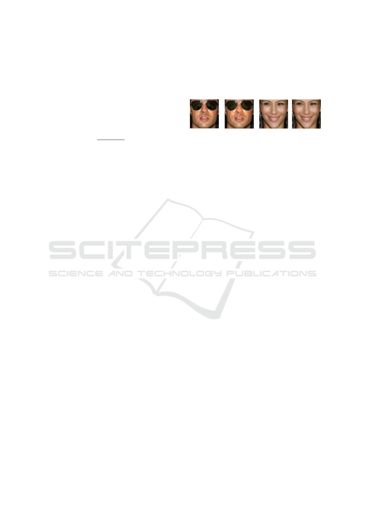
Figure 4: (b) and (d) show the results obtained after ap-

plying Poisson editing (equation (9) in the text) to the in-

painting results shown in (a) and (c), respectively.

The parameters α, β and η in equation (4) allow

to balance among the three losses. The selected pa-

rameters are α = 0.1, β = 1 − α and η = 0.5 but

for the sake of a thorough analysis we present in Ta-

bles 1 and 2 an ablation study of our contributions.

With the deﬁned contextual, gradient and prior los-

ses, the corrupted image can be mapped to the clo-

sest z in the latent representation space, denoted by

ˆz. z is randomly initialized with Gaussian noise of

zero mean and unit standard deviation and updated

using back-propagation on the total loss given in the

equation (4). Once G(ˆz) is generated, the inpainting

result can be obtained by overlaying the uncorrupted

pixels of the original damaged image to the generated

image. Even so, the reconstructed pixels may not ex-

actly preserve the same intensities of the surrounding

pixels although the content and structure is correctly

well aligned. To solve this problem, a Poisson editing

step (P

erez et al., ) is added at the end of the pipeline

in order to reserve the gradients of G(ˆz) without mis-

matching intensities of the input image y. Thus, the

ﬁnal reconstructed image ˆx is equal to:

ˆx = argmin

k∇x − ∇G(ˆz)k

such that x(i) = y(i) if M(i) = 1

(9)

Figure 4 shows an example where visible seams are

appreciated in (a) and (c), but less in (b) and (d) after

applying (9).

4 EXPERIMENTAL RESULTS

In this section we evaluate the proposed method both

qualitatively and quantitatively by using different eva-

luation metrics. We compare our results with the re-

sults obtained by (Yeh et al., 2017) as both algorithms

use ﬁrst a GAN procedure to learn semantic informa-

tion from a dataset and, second, combine it with an

VISAPP 2019 - 14th International Conference on Computer Vision Theory and Applications

254

(a)

(b)

(c)

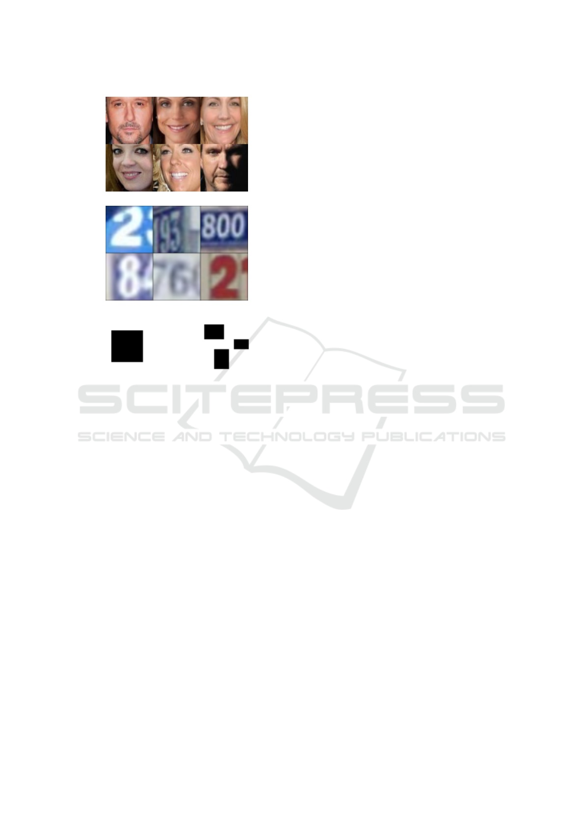
Figure 5: (a) Samples from CelebA training dataset. (b)

Samples from SVHN training dataset. (c) Two masks M

used in our experiments corresponding to different corrup-

ted regions (the black pixels): A central square on the left

and three rectangular areas on the right.

optimization loss for inpainting in order to infer the

missing content. In order to perform an ablation study

of all our contributions, we present the results obtai-

ned not only by using the original algorithm by (Yeh

et al., 2017) but also the results obtained by adding

our new gradient-based term L

(z|y, M) to their origi-

nal inpainting loss, and varying the trade-off between

the different loss terms (weights α, β, η).

In the training step of our algorithm, we use the

proposed architecture (see Section 3.1) where the

generative model takes a random vector, of dimen-

sion 128, drawn from a normal distribution. In con-

trast, (Yeh et al., 2017) uses the DCGAN architec-

ture where the generative model takes a random 100

dimensional vector following a uniform distribution

between [−1, 1]. For all the experiments we use: A

ﬁxed number of iterations equal to 50000, batch size

equal to 64, learning rate equal to 0.0001 and expo-

nential decay rate for the ﬁrst and second moment es-

timates in the Adam update technique, β

= 0, 0 and

= 0, 9, respectively. To increase the amount of trai-

ning data we also performed data augmentation by

randomly applying a horizontal ﬂipping on the trai-

ning set. Training the generative model required three

days using an NVIDIA TITAN X GPU.

In the inpainting step, the window size used to

compute W(i) in (5) is ﬁxed to 7x7 pixels. In our al-

gorithm, we use back-propagation to compute ˆz in the

latent space. We make use of an Adam optimizer and

restrict z to [−1, 1] in each iteration, which we found

it produces more stable results. In that stage we used

the Adam hyperparameters learning rate, α, equal to

0.03 and the exponential decay rate for the ﬁrst and

second moment estimates, β

= 0, 9 and β

= 0, 999,

respectively. After initializing with a random 128 di-

mensional vector z drawn from a normal distribution,

we perform 1000 iterations.

The assessment is given on two different data-

sets in order to check the robustness of our method:

the CelebFaces Attributes Datases (Liu et al., 2015)

and the Street View House Numbers (SVHN) (Netzer

et al., ). CelebA dataset contains a total of 202.599

celebrity images covering large pose variations and

background clutter. We split them into two groups:

201,599 for training and 1,000 for testing. In con-

trast, SVHN contains only 73,257 training images

and 26,032 testing images. SVHN images are not

aligned and have different shapes, sizes and back-

grounds. The images of both datasets have been crop-

ped with the provided bounding boxes and resized to

only 64x64 pixel size. Figure 5(a)-(b) displays some

samples from these datasets.

Let us remark that we have trained the proposed

improved WGAN by using directly the images from

the datasets without any mask application. After-

wards, our semanting inpainting method is evaluated

on both datasets using the inpainting masks illustra-

ted in Figure 5(c). Notice that our algorithm can be

applied to any type of inpainting mask.

Qualitative Assessment. We separately analyze each

step of our algorithm: The training of the genera-

tive model and the minimization procedure to infer

the missing content. Since the inpainting optimum of

the latter strongly depends on what the generative mo-

del is able to produce, a good estimation of the data

latent space is crucial for our task. Figure 6 shows

some images generated by our generative model trai-

ned with the CelebA and SVHN, respectively. Notice

that the CelebA dataset is better estimated due to the

fact that the number of images as well as the diver-

sity of the dataset directly affects the prediction of the

latent space and the estimated underlying probability

density function (pdf). In contrast, as bigger the va-

riability of the dataset, more spread is the pdf which

difﬁcult its estimation.

To evaluate our inpainting method we compare it

Semantic Image Inpainting through Improved Wasserstein Generative Adversarial Networks

255

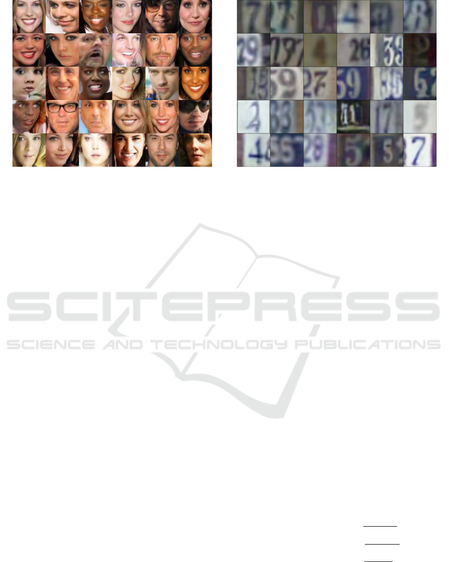
Figure 6: Some images generated by our generative model using the CelebA and the SVHN dataset as training set, respectively.

The CelebA dataset contains around 200k training images which are aligned and preprocessed to reduce the diversity between

samples. The SVHN dataset contains 73.257 training images. In this case, no pre-processing to reduce the diversity between

samples has been applied. Notice that both datasets have been down-sampled to 64x64 pixel size before training.

with the semantic inpainting method of (Yeh et al.,

2017). Some qualitative results are displayed in Figu-

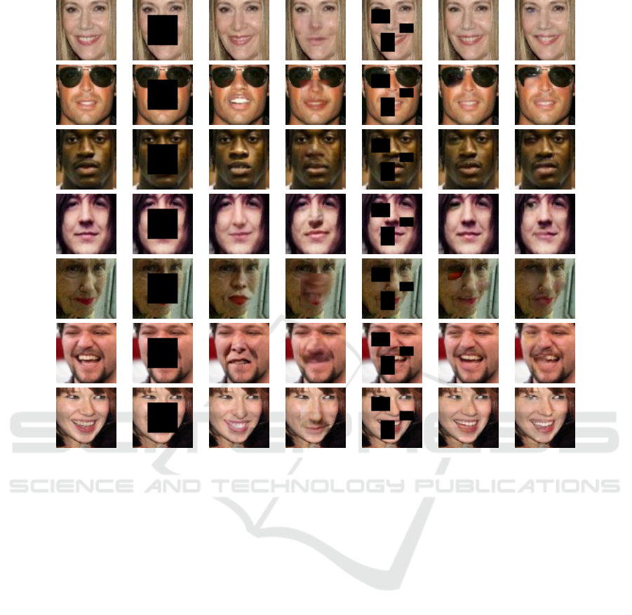
res 7 and 8. Focusing on the CelebA results (Figure

7), obviously (Yeh et al., 2017) performs much better

than local and non-local methods (Figure 2) since it

also makes use of generative models. However, alt-

hough that method is able to recover the semantic in-

formation of the image and infer the content of the

missing areas, in some cases it keeps producing re-

sults with lack of structure and detail which can be

caused either by the generative model or by the proce-

dure to search the closest encoding in the latent space.

We will further analyze it with a quantitative ablation

study of our contributions. Since our method takes

into account not only the pixel values but also the

structure of the image this kind of problems are sol-

ved. In many cases, our results are as realistic as the

real images. Notice that challenging examples, such

as the ﬁfth image from Figure 7, which image struc-

tures are not well deﬁned, are not properly recovered

with our method nor with (Yeh et al., 2017). Some

failure examples are shown in Figure 9.

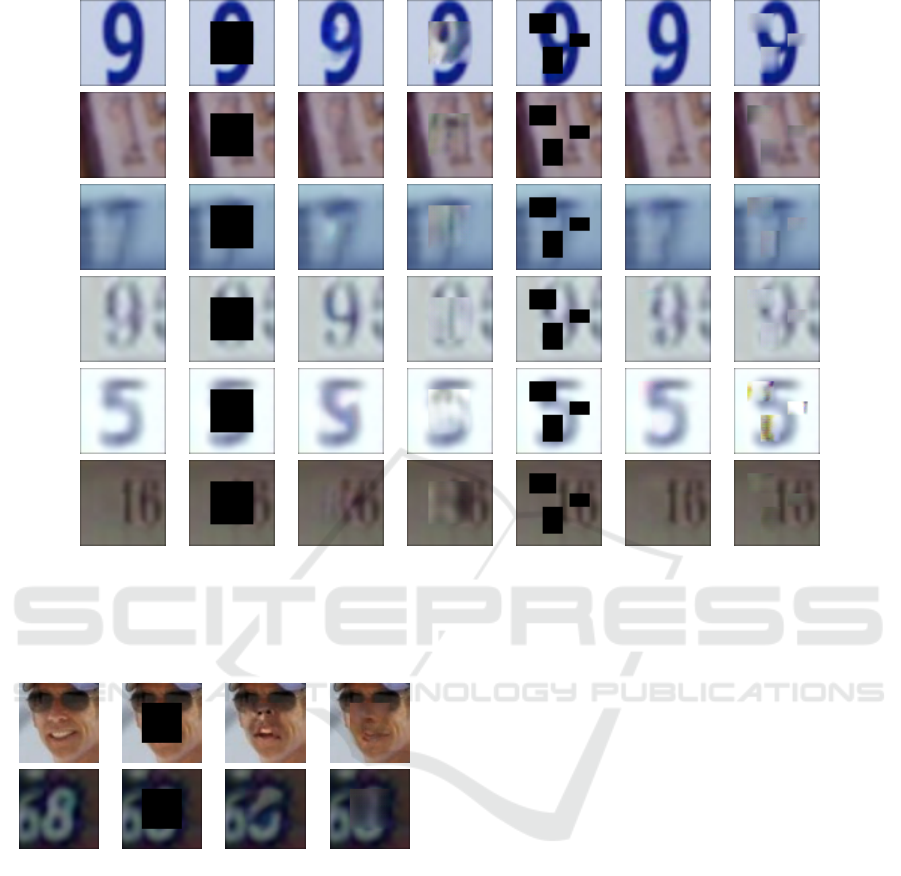
Regarding the results on SVHN dataset (Figure 8),

although they are not as realistic as the CelebA ones,

the missing content is well recovered even when dif-

ferent numbers may semantically ﬁt the context. As

mentioned before, the lack of detail is probably cau-

sed by the training stage, due to the large variability

of the dataset (and the small number of examples).

Despite of this, let us notice that our qualitative re-

sults outperform the ones of (Yeh et al., 2017). This

may indicate that our algorithm is more robust in the

case of smaller datasets than (Yeh et al., 2017).

Quantitative Analysis and Evaluation Metrics.

The goal of semantic inpainting is to ﬁll-in the mis-

sing information with realistic content. However,

with this purpose, there are many correct possibilities

to semantically ﬁll the missing information. In ot-

her words, a reconstructed image equal to the ground

truth would be only one of the several potential solu-

tions. Thus, in order to quantify the quality of our

method in comparison with other methods, we use

different evaluation metrics: First, metrics based on a

distance with respect to the ground truth and, second,

a perceptual quality measure that is acknowledged to

agree with similarity perception in the human visual

system.

In the ﬁrst case, considering the real images from

the database as the ground truth reference, the most

used evaluation metrics are the Peak Signal-to-Noise

Ratio (PSNR) and the Mean Square Error (MSE).

Notice, that both MSE and PSNR, will choose as

best results the ones with pixel values closer to the

ground truth. In the second case, in order to evaluate

perceived quality, we use the Structural Similarity in-

dex (SSIM) (Wang et al., 2004) used to measure the

similarity between two images. It is considered to be

correlated with the quality perception of the human

visual system and is deﬁned as:

SSIM(x, y) = l(x, y) · c(x, y) · s( f , g)

where











l(x, y) =

2µ

+µ

c(x, y) =

2σ

+σ

s(x, y) =

2σ

(10)

The ﬁrst term in (10) is the luminance comparison

function which measures the closeness of the two

images mean luminance (µ

and µ

). The second term

is the contrast comparison function which measures

VISAPP 2019 - 14th International Conference on Computer Vision Theory and Applications

256

Original Masked Ours SIMDGM Masked Ours SIMDGM

Figure 7: Inpainting results on the CelebA dataset: Qualitative comparison with the method (Yeh et al., 2017) (fourth and

seventh columns, referenced as SIMDGM), using the two masks shown in the second and ﬁfth columns, is also displayed.

the closeness of the contrast of the two images, where

, σ

denote the standard deviations. The third term

is the structure comparison function which measures

the correlation between x and y. C

and C

are

small positive constants avoiding dividing by zero.

Finally, σ

denotes the covariance between x and y.

The SSIM is maximal when is equal to one.

Given these metrics we compare our results with

the one proposed by (Yeh et al., 2017) as it is the met-

hod more similar to ours. Tables 1 and 2 show the

numerical performance of our method and (Yeh et al.,

2017) using both the right and left inpainting masks

shown in Figure 5(c), respectively, named from now

on, central square and three squares mask, respecti-

vely. To perform an ablation study of all our contri-

butions and a complete comparison with (Yeh et al.,

2017), Tables 1 and 2 not only show the results obtai-

ned by their original algorithm and our proposed al-

gorithm, but also the results obtained by adding our

new gradient-based term L

(z|y, M) to their original

inpainting loss. We present the results varying the

trade-off effect between the different loss terms.

Our algorithm always performs better than the se-

mantic inpainting method by (Yeh et al., 2017). For

the case of the CelebA dataset, the average MSE

obtained by (Yeh et al., 2017) is equal to 872.8672

and 622.1092, respectively, compared to our results

that are equal to 785.2562 and 321.3023, respecti-

vely. It is highly reﬂected in the results obtained using

the SVHN dataset, where the original version of (Yeh

et al., 2017) obtains an MSE equal to 1535.8693 and

1531.4601, using the central and three squares mask

respectively, and our method 622.9391 and 154.5582.

On the one side, the proposed WGAN structure is able

to create a more realistic latent space and, on the ot-

her side, the proposed loss takes into account essential

information in order to recover the missing areas.

Regarding the accuracy results obtained with the

SSIM measure, we can see that ours results always

have a better perceived quality than the ones obtained

by (Yeh et al., 2017). In some cases, the values are

close to the double, for example, in the case of using

the dataset SVHN.

We can also conclude that our method is more sta-

Semantic Image Inpainting through Improved Wasserstein Generative Adversarial Networks

257

Original Masked Ours SIMDGM Masked Ours SIMDGM

Figure 8: Inpainting results on the SVHN dataset: Qualitative comparison with the method (Yeh et al., 2017) (fourth and

seventh columns, referenced as SIMDGM), using the two masks shown in the second and ﬁfth columns, is also displayed.

Original Masked Ours SIMDGM

Figure 9: Some examples of failure cases.

ble in smaller datasets such in the case of SVHN. In

our case, decreasing the number of samples in the da-

taset does not mean to reduce the quality of the in-

painted images. Contrary with what is happening in

the case of (Yeh et al., 2017). Finally, in the cases

where we add the proposed loss to the algorithm pro-

posed by (Yeh et al., 2017), in most of the cases the

MSE, PSNR and SSIM improves. This fact clariﬁes

the big importance of the gradient loss in order to per-

form semantic inpainting.

5 CONCLUSIONS

In this work we propose a new method that takes ad-

vantage of generative adversarial networks to perform

semantic inpainting in order to recover large missing

areas of an image. This is possible thanks to, ﬁrst, an

improved version of the Wasserstein Generative Ad-

versarial Network which is trained to learn the latent

data manifold. Our proposal includes a new genera-

tor and discriminator architectures having stabilizing

properties. Second, we propose a new optimization

loss in the context of semantic inpainting which is

able to properly infer the missing content by condi-

tioning to the available data on the image, through

both the pixel values and the image structure, while

taking into account the perceptual realism of the com-

plete image. Our qualitative and quantitative experi-

ments demostrate that the proposed method can infer

more meaningful content for incomplete images than

local, non-local and semantic inpainting methods. In

particular, our method qualitatively and quantitatively

outperforms the related semantic inpainting method

(Yeh et al., 2017) obtaining images with sharper ed-

ges, which looks like more natural and perceptually

similar to the ground truth.

VISAPP 2019 - 14th International Conference on Computer Vision Theory and Applications

258

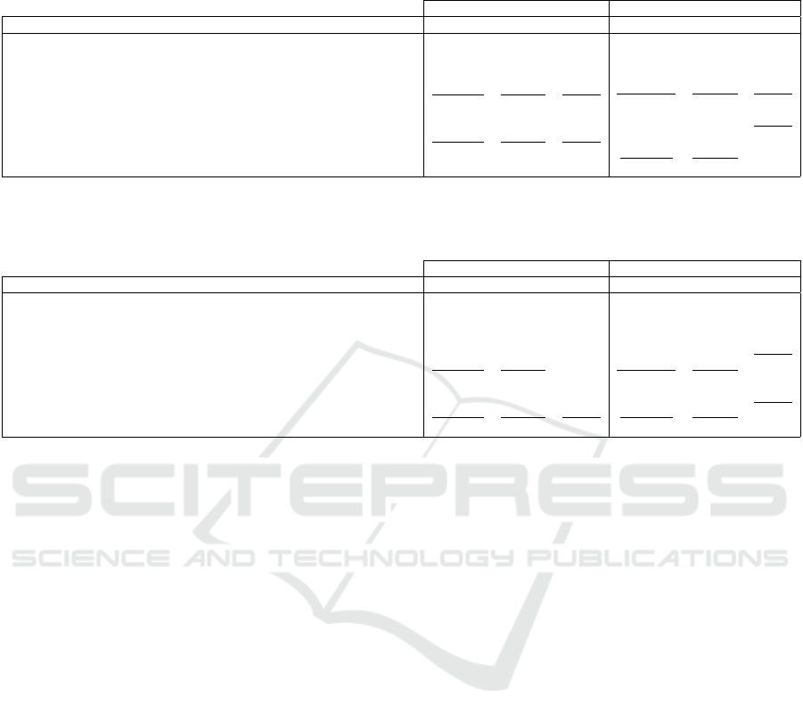
Table 1: Quantitative inpainting results for the central square mask (shown in Fig. 5(c)-left), including an ablation study of

our contributions in comparison with (Yeh et al., 2017). The best results for each dataset are marked in bold and the best

results for each method are underlined.

CelebA dataset SVHN dataset

Loss formulation MSE PSNR SSIM MSE PSNR SSIM

(Yeh et al., 2017) 872.8672 18.7213 0.9071 1535.8693 16.2673 0.4925

(Yeh et al., 2017) adding gradient loss with α = 0.1, β = 0.9 and η = 1.0 832.9295 18.9247 0.9087 1566.8592 16.1805 0.4775

(Yeh et al., 2017) adding gradient loss with α = 0.5, β = 0.5 and η = 1.0 862.9393 18.7710 0.9117 1635.2378 15.9950 0.4931

(Yeh et al., 2017) adding gradient loss with α = 0.1, β = 0.9 and η = 0.5 794.3374 19.1308 0.9130 1472.6770 16.4438 0.5041

(Yeh et al., 2017) adding gradient loss with α = 0.5, β = 0.5 and η = 0.5 876.9104 18.7013 0.9063 1587.2998 16.1242 0.4818

Our proposed loss with α = 0.1, β = 0.9 and η = 1.0 855.3476 18.8094 0.9158 631.0078 20.1305 0.8169

Our proposed loss with α = 0.5, β = 0.5 and η = 1.0 785.2562 19.1807 0.9196 743.8718 19.4158 0.8030

Our proposed loss with α = 0.1, β = 0.9 and η = 0.5 862.4890 18.7733 0.9135 622.9391 20.1863 0.8005

Our proposed loss with α = 0.5, β = 0.5 and η = 0.5 833.9951 18.9192 0.9146 703.8026 19.6563 0.8000

Table 2: Quantitative inpainting results for the three squares mask (shown in Fig. 5(c)-right), including an ablation study of

our contributions and a complete comparison with (Yeh et al., 2017). The best results for each dataset are marked in bold and

the best results for each method are underlined.

CelebA dataset SVHN dataset

Method MSE PSNR SSIM MSE PSNR SSIM

(Yeh et al., 2017) 622.1092 20.1921 0.9087 1531.4601 16.2797 0.4791

(Yeh et al., 2017) adding gradient loss with α = 0.1, β = 0.9 and η = 1.0 584.3051 20.4644 0.9067 1413.7107 16.6272 0.4875

(Yeh et al., 2017) adding gradient loss with α = 0.5, β = 0.5 and η = 1.0 600.9579 20.3424 0.9080 1427.5251 16.5850 0.4889

(Yeh et al., 2017) adding gradient loss with α = 0.1, β = 0.9 and η = 0.5 580.8126 20.4904 0.9115 1446.3560 16.5281 0.5120

(Yeh et al., 2017) adding gradient loss with α = 0.5, β = 0.5 and η = 0.5 563.4620 20.6222 0.9103 1329.8546 16.8928 0.4974

Our proposed loss with α = 0.1, β = 0.9 and η = 1.0 424.7942 21.8490 0.9281 168.9121 25.8542 0.8960

Our proposed loss with α = 0.5, β = 0.5 and η = 1.0 380.4035 22.3284 0.9314 221.7906 24.6714 0.9018

Our proposed loss with α = 0.1, β = 0.9 and η = 0.5 321.3023 23.0617 0.9341 154.5582 26.2399 0.8969

Our proposed loss with α = 0.5, β = 0.5 and η = 0.5 411.8664 21.9832 0.9292 171.7974 25.7806 0.8939

Unsupervised learning needs enough training data

to learn the distribution of the data and generate re-

alistic images to eventually succeed in semantic in-

painting. A huge dabaset with higher resolution ima-

ges would be needed to apply our method to more

complex and diverse world scenes. The presented re-

sults are based on low resolution images (64x64 pixel

size) and thus the inpainting method is limited to ima-

ges of that resolution. Also, more complex features

needed to represent such complex and diverse world

scenes would require a deeper architecture. Future

work will follow these guidelines.

ACKNOWLEDGEMENTS

The authors acknowledge partial support by MI-

NECO/FEDER UE project, reference TIN2015-

70410-C2-1 and by H2020-MSCA-RISE-2017 pro-

ject, reference 777826 NoMADS.

REFERENCES

Adler, J. and Lunz, S. (2018). Banach wasserstein gan.

arXiv:1806.06621.

Arias, P., Facciolo, G., Caselles, V., and Sapiro, G. A vari-

ational framework for exemplar-based image inpain-

ting. IJCV.

Arjovsky, M., Chintala, S., and Bottou, L. (2017). Wasser-

stein gan. arXiv:1701.07875.

Aujol, J.-F., Ladjal, S., and Masnou, S. (2010).

Exemplar-based inpainting from a variational point

of view. SIAM Journal on Mathematical Analysis,

42(3):1246–1285.

Ba, J. L., Kiros, J. R., and Hinton, G. E. (2016). Layer

normalization. arXiv:1607.06450.

Ballester, C., Bertalm

ıo, M., Caselles, V., Sapiro, G., and

Verdera, J. (2001). Filling-in by joint interpolation

of vector ﬁelds and gray levels. IEEE Trans. on IP,

10(8):1200–1211.

Burlin, C., Le Calonnec, Y., and Duperier, L. (2017). Deep

image inpainting.

Cao, F., Gousseau, Y., Masnou, S., and P

erez, P. (2011). Ge-

ometrically guided exemplar-based inpainting. SIAM

Journal on Imaging Sciences, 4(4):1143–1179.

Cao, Y. e. a. (2017). Unsupervised diverse colorization via

generative adversarial networks. In Machine Learning

and Knowledge Discovery in Databases. Springer.

Chan, C., Ginosar, S., Zhou, T., and Efros, A. A. (2018).

Everybody dance now. arXiv:1808.07371.

Chan, T. and Shen, J. H. (2001). Mathematical models for

local nontexture inpaintings. SIAM Journal of App-

lied Mathematics, 62(3):1019–1043.

Criminisi, A., P

erez, P., and Toyama, K. (2004). Region ﬁl-

ling and object removal by exemplar-based inpainting.

IEEE Trans. on IP, 13(9):1200–1212.

Demanet, L., Song, B., and Chan, T. (2003). Image inpain-

ting by correspondence maps: a deterministic appro-

ach. App and Comp Mathematics, 1100:217–50.

Semantic Image Inpainting through Improved Wasserstein Generative Adversarial Networks

259

Demir, U. and

Unal, G. B. (2018). Patch-based image in-

painting with generative adversarial networks. CoRR,

abs/1803.07422.

Efros, A. A. and Leung, T. K. (1999). Texture synthesis by

non-parametric sampling. In ICCV, page 1033.

Fedorov, V., Arias, P., Facciolo, G., and Ballester, C. (2016).

Afﬁne invariant self-similarity for exemplar-based in-

painting. In Proceedings of the 11th Joint Conference

on Computer Vision, Imaging and Computer Graphics

Theory and Applications, pages 48–58.

Fedorov, V., Facciolo, G., and Arias, P. (2015). Variational

Framework for Non-Local Inpainting. Image Proces-

sing On Line, 5:362–386.

Getreuer, P. (2012). Total Variation Inpainting using Split

Bregman. Image Processing On Line, 2:147–157.

Goodfellow, I., Pouget-Abadie, J., Mirza, M., Xu, B.,

Warde-Farley, D., Ozair, S., Courville, A., and Ben-

gio, Y. (2014). Generative adversarial nets. In Adv in

neural inf processing systems, pages 2672–2680.

Gulrajani, I., Ahmed, F., Arjovsky, M., Dumoulin, V., and

Courville, A. C. (2017). Improved training of wasser-

stein gans. In Adv in Neural Inf Processing Systems,

pages 5769–5779.

He, K., Zhang, X., Ren, S., and Sun, J. (2016). Deep resi-

dual learning for image recognition. In CVPR.

Huang, J. B., Kang, S. B., Ahuja, N., and Kopf, J. (2014).

Image completion using planar structure guidance.

ACM SIGGRAPH 2014, 33(4):129:1–129:10.

Iizuka, S., Simo-Serra, E., and Ishikawa, H. (2017). Glo-

bally and locally consistent image completion. ACM

Trans. Graph., 36(4):107:1–107:14.

Kawai, N., Sato, T., and Yokoya, N. (2009). Image inpain-

ting considering brightness change and spatial locality

of textures and its evaluation. In Adv in Image and Vi-

deo Technology, pages 271–282.

Kingma, D. P. and Welling, M. (2013). Auto-encoding va-

riational bayes. arXiv:1312.6114.

Ledig, C., Theis, L., Husz

ar, F., Caballero, J., Cunning-

ham, A., Acosta, A., Aitken, A. P., Tejani, A., Totz,

J., Wang, Z., et al. (2017). Photo-realistic single

image super-resolution using a generative adversarial

network. In CVPR, volume 2, page 4.

Li, Y., Liu, S., Yang, J., and Yang, M.-H. (2017). Generative

face completion. In CVPR, volume 1, page 3.

Liu, M.-Y., Breuel, T., and Kautz, J. (2017). Unsupervi-

sed image-to-image translation networks. In Adv in

Neural Inf Processing Systems, pages 700–708.

Liu, Z., Luo, P., Wang, X., and Tang, X. (2015). Deep lear-

ning face attributes in the wild. In ICCV.

Mao, X., Li, Q., Xie, H., Lau, R. Y., Wang, Z., and Smol-

ley, S. P. (2017). Least squares generative adversarial

networks. In ICCV, pages 2813–2821.

Masnou, S. and Morel, J.-M. (1998). Level lines based

disocclusion. In Proc. of IEEE ICIP.

Netzer, Y., Wang, T., Coates, A., Bissacco, A., Wu, B., and

Ng, A. Y. Reading digits in natural images with unsu-

pervised feature learning. In NIPS workshop on deep

learning and unsupervised feature learning.

Nguyen, A., Yosinski, J., Bengio, Y., Dosovitskiy, A., and

Clune, J. (2016). Plug & play generative networks:

Conditional iterative generation of images in latent

space. arXiv:1612.00005.

Pathak, D., Krahenbuhl, P., Donahue, J., Darrell, T., and

Efros, A. A. (2016). Context encoders: Feature lear-

ning by inpainting. In CVPR.

erez, P., Gangnet, M., and Blake, A. Poisson image edi-

ting. In ACM SIGGRAPH 2003.

Pumarola, A., Agudo, A., Sanfeliu, A., and Moreno-

Noguer, F. (2018). Unsupervised Person Image Synt-

hesis in Arbitrary Poses. In CVPR.

Radford, A., Metz, L., and Chintala, S. (2015). Unsuper-

vised representation learning with deep convolutional

generative adversarial networks. arXiv:1511.06434.

Reed, S., Akata, Z., Yan, X., Logeswaran, L., Schiele, B.,

and Lee, H. (2016). Generative adversarial text to

image synthesis. In Proceedings of The 33rd Intern.

Conf. Machine Learning, pages 1060–1069.

Salimans, T., Goodfellow, I., Zaremba, W., Cheung, V.,

Radford, A., Chen, X., and Chen, X. Improved techni-

ques for training gans. In Adv in Neural Inf Processing

Systems 29.

van den Oord, A., Kalchbrenner, N., Espeholt, L., kavuk-

cuoglu, k., Vinyals, O., and Graves, A. Conditional

image generation with pixelcnn decoders. In Adv in

Neural Inf Processing Systems 29.

Wang, T.-C., Liu, M.-Y., Zhu, J.-Y., Tao, A., Kautz, J., and

Catanzaro, B. High-resolution image synthesis and se-

mantic manipulation with conditional gans. In CVPR.

Wang, Z. (2008). Image afﬁne inpainting. In Image Analy-

sis and Recognition, volume 5112 of Lecture Notes in

Computer Science, pages 1061–1070.

Wang, Z., Bovik, A. C., Sheikh, H. R., and Simoncelli,

E. P. (2004). Image quality assessment: from error

visibility to structural similarity. IEEE Trans. on IP,

13(4):600–612.

Yang, C., Lu, X., Lin, Z., Shechtman, E., Wang, O., and

Li, H. (2017). High-resolution image inpainting using

multi-scale neural patch synthesis. In CVPR, vo-

lume 1, page 3.

Yeh, R. A., Chen, C., Lim, T.-Y., Schwing, A. G.,

Hasegawa-Johnson, M., and Do, M. N. (2017). Se-

mantic image inpainting with deep generative models.

In CVPR, volume 2, page 4.

Yu, J., Lin, Z., Yang, J., Shen, X., Lu, X., and Huang, T. S.

Generative image inpainting with contextual attention.

Zhu, J.-Y., Park, T., Isola, P., and Efros, A. A. (2017a).

Unpaired image-to-image translation using cycle-

consistent adversarial networks. arXiv preprint.

Zhu, J.-Y., Park, T., Isola, P., and Efros, A. A. (2017b).

Unpaired image-to-image translation using cycle-

consistent adversarial networks. In ICCV.

VISAPP 2019 - 14th International Conference on Computer Vision Theory and Applications

260