
Detecting Anomalies by using Self-Organizing Maps in Industrial
Environments
Ricardo Hormann and Eric Fischer
Shopfloor IT, Volkswagen AG, Wolfsburg, Germany
Keywords:
Anomaly Detection, Self-Organizing Maps, Profinet.
Abstract:
Detecting anomalies caused by intruders are a big challenge in industrial environments due to the complex
environmental interdependencies and proprietary fieldbus protocols. In this paper, we proposed a network-
based method for detecting anomalies by using unsupervised artificial neural networks called Self-Organizing
Maps (SOMs). Therefore, we published an algorithm which identifies clusters and cluster centroids in SOMs
to gain knowledge about the underlying data structure. In the training phase we created two neural networks,
one for clustering the network data and the other one for finding the cluster centroids. In the operating phase
our approach is able to detect anomalies by comparing new data samples with the first trained SOM model.
We used a confidence interval to decide if the sample is too far from its best matching unit. A novel additional
confidence interval for the second SOM is proposed to minimize false positives which have been a major
drawback of machine learning methods in anomaly detection. We implemented our approach in a robot cell
and infiltrated the network like an intruder would do to evaluate our method. As a result, we significantly
reduced the false positive rate to 0.07% using the second interval while providing an accuracy of 99% for the
detection of network attacks.
1 INTRODUCTION
Traditionally, industrial communication networks are
isolated systems that usually only allow internal com-
munication. Recent developments within the Industry
4.0 show the trend towards using more information
and communication technologies (ICT) in industrial
control systems (ICS) (Schuster et al., 2013). Many
field devices and protocols currently in use have been
originally designed for isolated and highly trusted au-
tomation networks with a physical air gap to other
networks. As cyber security has not been taken into
account during their development, these systems lack
essential IT security features. This design decision is
not compatible with the nowadays often implemented
connection to more open and thus less trusted net-
works like supervisory networks that use open pro-
tocols (e.g. TCP/IP) (Knapp, 2011).
With these new interfaces, more attack possibili-
ties emerge with an increased damage potential like
“Stuxnet” in 2010 (Langner, 2011) and “WannaCry”
in 2017 (Ehrenfeld, 2017). The steadily increasing
complexity of automation networks indicates the ne-
cessity of more advanced intrusion detection systems
(IDS) that do not exclusively rely on searching for
signa-
tures that characterize previously known attacks.
There is a need for IDSs that also identify unknown
threats (zero-day attacks). Due to the general lack of
carefully labeled data sets in complex communication
networks, unsupervised machine learning algorithms
like Self-Organizing Maps (SOMs) are suitable meth-
ods for such IDS (Ippoliti and Zhou, 2012). They aim
at constructing a model characterizing normal behav-
ior of a system by extracting raw data during normal
operation (Di Pietro and Mancini, 2008).
These aspects motivate the analysis of industrial
networks using SOMs to detect anomalies that indi-
cate security relevant incidents. The general prob-
lem of too many false alarms of anomaly-based IDS
should be addressed to make them attractive for prac-
tical use. Taking the above into account, this paper
proposes a concept for the analysis of SOMs to facil-
itate the detection of outliers in ICS.
2 INDUSTRIAL CONTROL
SYSTEMS
Industrial control systems describe networks that op-
erate and manage industrial processes such as an
336
Hormann, R. and Fischer, E.
Detecting Anomalies by using Self-Organizing Maps in Industrial Environments.
DOI: 10.5220/0007364803360344
In Proceedings of the 5th International Conference on Information Systems Security and Privacy (ICISSP 2019), pages 336-344
ISBN: 978-989-758-359-9
Copyright
c
2019 by SCITEPRESS – Science and Technology Publications, Lda. All rights reserved

automated manufacturing step in an automotive as-
sembly line. ICSs utilize a real-time communica-
tion between their devices through fieldbuses and in-
dustrial Ethernet protocols (Knapp, 2011). ICSs are
located in production cells and contain control de-
vices such as programmable logic controllers (PLCs)
to operate machines and robots and human-machine
interfaces (HMI) for monitoring and manual adjust-
ments (Stouffer et al., 2011; Knapp, 2011). Further,
PLCs can be connected to fieldbuses that link field
devices like sensors, motors and valves at shop floor
level. Different network zones ensure that devices in
the corporate network cannot communicate directly
with the control network and vice versa which is im-
portant as the networks have different trust levels.
Profinet is a real-time capable Ethernet-based
communication protocol and was invented in the
1980s to facilitate fast and reliable data exchange be-
tween controlling units and field devices. There are
mainly two different classes of Profinet communica-
tion: Profinet CBA to transmit non time critical data
and Profinet IO for the cyclic and non cyclic data ex-
change in real time between IO controllers (PLCs)
and IO devices (field devices). Profinet IO (PNIO)
itself consists of several sub-protocols. To setup a
Profinet communication, the PNIO-Context Manager
(PNIO-CM) is used. It bases on UDP and establishes
the initial PNIO connection. The actual cyclic sta-
tus data is exchanged as PNIO packets via Ethernet
frames on OSI layer 2 and is not acknowledged. Each
Profinet data unit is directly embedded in an Ether-
net frame and directed from one node to another via
the MAC addresses of the communicating devices. Its
payload contains status information and IO data val-
ues whose meanings are negotiated by PNIO-CM in
the communication setup. The data exchange is struc-
tured as a publish/subscribe model where the IO con-
troller can subscribe to information published by IO
devices. Further, Profinet IO also supports non cyclic
communication for alarm messages in form of PNIO-
AL (Frank, 2009).
3 SELF-ORGANIZING MAPS
A Self-Organizing Map is an artificial neural net-
work (ANN) that receives high dimensional data as
an input and learns its complex structures to repre-
sent it on a two dimensional map of neurons as the
output. It behaves like a dynamic and flexible lat-
tice that is spanned over the input data samples to
approximate it as shown in Fig. 1 on the left hand
side. In other words it fits two-dimensionally ordered
prototype vectors to the distribution of the high di-
mensional input data vectors (Kohonen et al., 2001).
The method is inspired by the functionality of the hu-
man brain where similar inputs activate neurons in the
same area of the brain. Thus, data instances that are
close in the input data space are mapped to neurons
that are nearby on the output map. This property is
called topological correctness and makes the SOM a
unique and useful tool for exploring data sets as it vi-
sually represents high dimensional data. Further, the
SOM does not require manually labeled data sets as
an input and can be classified as an unsupervised ma-
chine learning method. Originally, the algorithm was
introduced by the Finnish researcher Teuvo Kohonen
in 1982 (Kohonen, 1982) and has been successfully
used in well over 10000 publications until 2011 (Ko-
honen et al., 2001).
3.1 Algorithm
The original SOM algorithm essentially consists of
four steps. First, a usually two dimensional lattice of
neurons like in Fig. 1 is initialized by creating a vec-
tor for each neuron that has certain coordinates on the
map. The dimension of each of those prototype vec-
tors has to match with the later used input data vec-
tors. The values of each prototype vector can be ini-
tialized randomly or in a linear way according to the
minimum and maximum values of each vector com-
ponent in the training data.
The second phase can be called competition phase
as the neurons compete for each input that is pre-
sented to the neural network to be selected as the win-
ner neuron. In Fig. 1 a training sample s is chosen
randomly from the input data set represented as a blue
cloud. Next, the input vector is compared to each pro-
totype vector on the map computing the distance be-
tween them (e.g. euclidean distance) and the one with
the smallest distance is chosen. Hence the winner is
also called best matching unit of s (BMU(s)) and rep-
resents it most accurately out of all neurons.
Figure 1: SOM algorithm and learning phase based on (Ko-
honen et al., 2001).
Thirdly, the winning neuron determines the topo-
logical area of the map that is ’activated’ by the input
s in the cooperation phase. Further, the grid structure
Detecting Anomalies by using Self-Organizing Maps in Industrial Environments
337

of the map defines the neighborhood neurons that are
stimulated along with its center node (the winner neu-
ron). In our case the three closest neurons are set as
the neighborhood of BMU(s).
Last is the adaption phase where the winning neu-
ron and its neighborhood adapt to the input. Given a
certain learning rate that decreases over time the stim-
ulated prototype vectors are ’shifted’ towards the in-
put vector so that their distances to the input decrease.
Hereby the degree of adaption is dependent on the
similarity of the current neuron to the input s so that
neighboring neurons adapt less than BMU(s). These
four steps are performed for each input training data
sample. After all samples have been applied to the
SOM one training iteration (called epoch) is finished.
The number of epochs that are performed until the al-
gorithm stops depends on the learning rate (Kohonen
et al., 2001).
3.2 U-Matrix and Clusters
A popular possibility to represent the SOM and its
topological cluster structures is the so called Unified
Distance Matrix (U-Matrix) introduced by (Ultsch,
1995). For each prototype vector of the SOM the av-
erage distance to its surrounding vectors is computed
and saved in a matrix structure preserving the respec-
tive map coordinate. Thus, low values in the U-Matrix
describe dense areas among the SOM i.e. neuron
clusters containing prototype vectors that are close to
each other characterize similar behavior. On the other
hand high distance values represent sparse areas in-
dicating outlying neurons. Moreover, when analyz-
ing cluster structures valuable information about the
underlying data can be extracted from the U-Matrix,
e.g. the number of clusters in the input data (Vesanto
and Alhoniemi, 2000) for further cluster algorithms
like k-means. In related research, (Brugger et al.,
2008) proposed an algorithm creating a clusot sur-
face to cluster data and to determine the number of
clusters. This method however is computationally
too expensive for our objective to identify the num-
ber of clusters as a first step of several analysis meth-
ods and anomaly detection. Other research introduced
a semi-automatic approach (Opolon and Moutarde,
2004) based on the U-Matrix to cluster the SOM neu-
rons by trial-and-error principle requiring manual in-
teraction. Thus, there is need for a fully automatic
algorithm that quickly computes a reliable reference
value approximating the number of clusters in a SOM.
This issue is addressed by a novel algorithm based on
the U-Matrix proposed in Section 4.1.
4 APPROACH
In this chapter a concept for analyzing Self-
Organizing Maps is proposed to detect anomalies and
to reduce false positives in the traffic of industrial con-
trol systems.
4.1 Cluster Analysis of Self-Organizing
Maps
The goal of this section is to gain knowledge about
the trained SOM to improve the detection accuracy of
outliers in the test data. First, a novel algorithm is
proposed that identifies the number of neuron clusters
present in a trained SOM model in Section 4.1.1. The
quality of the resulting clusters can be validated with
methods described in Section 4.1.2. In Section 4.1.3
the centroid vector of each neuron cluster is approxi-
mated.
4.1.1 Identifying Clusters
In general there is no ’right’ amount of clusters, but
a clustering quality metric can be used to find the
number that delivers the best performance consider-
ing that metric. Usually this is done by the trial-
and-error method. However, there is a significant
amount of possible cluster numbers when analyzing
high amounts of data occurring in communication
networks e.g. 160 is optimal in (Y
¨
uksel et al., 2016).
Thus, an algorithm that automatically computes the
approximated number of clusters can be useful and
saves time. In the following such an algorithm is pro-
posed that utilizes the structure of the U-Matrix of
a SOM to determine the number of existing neuron
clusters. It solely relies on the data provided in the
Unified Distance Matrix. Essentially, Alg. 1 tries to
find starting points for a cluster in the most dense ar-
eas of the map. When it finds an unused neuron it
scans the neighboring neurons i and adds them to the
current cluster j if they are close enough (see line 6 in
Alg. 1) meaning they fulfill Eq. (1)
1
. The algorithm
searches the U-Matrix like a depth-first-search regard-
ing the minimum U-Matrix value of the current clus-
ter members and neighbors. Moreover, if there are no
more potential nodes to add to the current cluster, it
validates the cluster depending on its size and density
compared to the map size of the SOM and global av-
erage density of the U-Matrix. Thus, if a found cluster
is too sparse or does not have enough members, it is
not accepted. These nodes may be added to a cluster
1
avg umat j is the average U-Matrix value for the cur-
rent cluster and σ
global umat dist
is the global standard devia-
tion of all U-Matrix values.
ICISSP 2019 - 5th International Conference on Information Systems Security and Privacy
338

in a future iteration of the algorithm, but they are not
forced to fit a cluster and some neurons may be left
unassigned at the end of the algorithm.
umat
i
<= avg umat j + σ
global umat dist
(1)
Algorithm 1: Textual description of the ’clus-
terfinder’ algorithm.
Input : Unified Distance Matrix of the
trained SOM model.
Output: Reference number of neuron
clusters in the SOM.
1 while Potential cluster starting points left do
2 From all neurons that are not part of any
cluster add the neuron with the smallest
U-Matrix value to the potential new
cluster and mark it as used
3 Add its neighboring unassigned neurons
to the potential member list
4 while Potential members left for the
current cluster do
5 current neuron ← get the one with the
current minimum U-Matrix value
from the potential neurons
6 if current neuron’s Umat value is
small enough then
7 add the neuron to the cluster and
add its neighbors to the potential
member list
8 else
9 remove neuron from the potential
members list
10 end
11 end
12 If the current cluster is valid then save it
13 end
14 Return the number of found valid clusters.
After finishing the clustering process the number
of clusters is returned which can be interpreted as a
reference number of the existing clusters in the SOM.
Reference means in this case that the cluster number
is validated by checking the numbers around that ref-
erence value as described in Section 4.1.2.
4.1.2 Confirming Cluster Quality
The ’cluster finder’ algorithm from Section 4.1.1 pro-
posed a possible number of neuron clusters k in the
SOM after analyzing the U-Matrix representation.
However, the quality of the resulting clustering has
to be verified as a next step using some kind of qual-
ity metric. To determine the ’right amount’ of clus-
ters, silhouette analysis is a widely accepted method
as the resulting silhouette score is only dependent on
the partition of the objects and not on the used cluster-
ing algorithm (Rousseeuw, 1987). Moreover, (Petro-
vic, 2006) show that silhouette analysis performs bet-
ter than an alternative metric like Davies Bouldin in
the context of anomaly IDS at cost of a more complex
and time consuming algorithm.
The silhouette score s of a single object i belong-
ing to some cluster is defined for k >= 2 in Eq. (2).
s(i) =
b(i) − a(i)
max(a(i), b(i))
(2)
Variable b(i) is the mean of all distances between
object i and the objects in its nearest cluster to which
i does not belong. Variable a(i) is the average dis-
tance between object i and all other objects that be-
long to the same cluster as object i. The single silhou-
ette scores s(i) ∈ [−1;1]
2
are averaged for all clusters
resulting in an overall average silhouette score ¯s(k).
A positive value near 1 means the clusters are (in av-
erage) really different to each other and objects of the
same cluster are similar. Ergo, the k with the highest
¯s(k) should be chosen (Rousseeuw, 1987).
In our concept, we evaluate ¯s(k) for several values
of k around the reference value that has been com-
puted by the ’cluster finder’ algorithm to save time
compared to a pure trial-and-error approach where k
increases for higher map sizes of the SOM.
4.1.3 Finding Cluster Centroids
As previously stated, the goal is to gain more knowl-
edge about the computed SOM representing normal
network behavior. By identifying its cluster centers
using an additional SOM layer, the distance of a test-
ing data sample to said centers can be a useful in-
formation for the decision if a data sample is normal
or anomalous. This is due to the clusters represent-
ing high values for the probability density function of
the input space (Kohonen, 2014). This is motivated
by following scenario illustrated in Fig. 2 where the
output space of a trained SOM is shown. There are
three clusters of neurons with their respective cluster
centroid vectors c1, c2 and c3. Let s1 be a normal
testing sample and s2 be an anomalous testing sam-
ple. The BMU distances (red lines) of both samples
are equal but s1 is quite similar to the normal behav-
iors of the three clusters compared to s2 which is a
significant outlier. In other words, the summed dis-
tances of s1 to the centroids are much smaller than
the summed distances of s2 to said centroids. If only
2
A negative value indicates the object i has been as-
signed to the wrong cluster and a value of 0 means the object
is right between the two clusters.
Detecting Anomalies by using Self-Organizing Maps in Industrial Environments
339
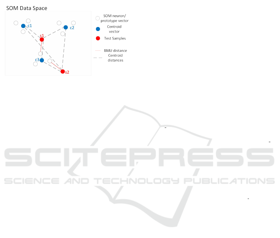
the BMU distance of a testing sample is considered,
valuable information might be lost. Therefore, con-
sidering the average cluster centroid distances in the
anomaly detection process could improve the detec-
tion performances.
Figure 2: SOM Clusters with two possible outliers.
To compute the centroid vectors of neuron clusters
of a SOM, the number of clusters has to be determined
before which is done in Section 4.1.1. Subsequently,
a second layer SOM - called cluster center SOM (CC-
SOM) in the following - can be trained to find the cen-
troids of the main SOM like in Fig. 2. The CCSOM’s
number of neurons equals the desired cluster number
(e.g. 3) while the training data remains the same as
for the main SOM. Consequently, the CCSOM tries
to represent the whole input space with the three cho-
sen neurons. The prototype vector of each neuron in
the output layer adapts to a specific cluster represent-
ing its centroid vector (Kohonen et al., 2001). On the
other hand, the centroid vectors could also be com-
puted using the k-means algorithm. However, since
it is prone to an initialization bias with its local op-
tima differing from the global optimum, the CCSOM
has been chosen to find fitting cluster centroids in the
initial try (Bac¸
˜
ao et al., 2005).
4.2 Detecting Anomalies
As the trained SOM represents the normal operating
state of the monitored network in our concept, we can
identify anomalous data samples by comparing them
to the SOM.
The first step is to compute a threshold δ
max
that
describes the acceptable degree of deviation from a
SOM neuron (its BMU). This can be done e.g. by
setting the maximum observed BMU distance as the
δ
max
. However, this value may be distorted due to the
training data being noisy in a real scenario. To filter
out this noise, one possible approach is to compute a
confidence interval I
bmu
= [0, δ
percentile
] during train-
ing that contains e.g. 99.99% of the BMU distance
values to the respective training samples (Bellas et al.,
2014). Further, for each testing sample x
i
the distance
to its BMU neuron d
bmu
(i) = d(x
i
, bmu(x
i
)) is com-
puted. If d
bmu
(i) ∈ I
bmu
then the testing data sample i
is classified as a normal packet. Else it is labeled as
an anomaly.
(Bellas et al., 2014) also introduced the idea to
construct a confidence interval for every SOM node’s
distance to its mapped training inputs. However, this
does not consider the nodes which were not cho-
sen as BMUs during the training phase but repre-
sent small deviations from other mapped neurons.
This together with the evaluation of (Goldstein and
Uchida, 2016) motivated the authors’ idea for the fol-
lowing. The summed distance to the cluster centroids
d
cent
may be useful as they represent dense points
of the input space (normal behavior) as explained in
Section 4.1.3. Also when training a SOM with an
anomaly in the training data, we observed that the
BMU of said anomaly is most of the time located at
the outside of the map as the anomaly differs signifi-
cantly from other inputs. Hence it has a high value for
d
cent
. The idea is to build a second confidence interval
I
centroid dist
which describes the summed distances of
a SOM neuron to the computed centroid vectors. If
d
cent
of a testing data sample is outside of I
centroid dist
,
the testing data sample is not located in between the
found clusters or around their neuron members and
thus rather outside like the sample s2 in Fig. 2. This
information is useful when the main confidence inter-
val I
bmu
barely identifies a sample as an anomaly, e.g.
it only exceeds the threshold δ
max
by a bit based on
the variance of the other distances. In other words,
it may be a false positive. Using I
centroid dist
as a sec-
ondary decision component can help to verify that the
anomalously classified testing sample is indeed intru-
sive.
5 IMPLEMENTATION
As a first step the collected raw network data is trans-
formed, because usually machine learning algorithms
require numerical values (Hormann et al., 2018). This
is critical if features are created per packet as the raw
data types depend on the spoken network protocol and
may not be of numerical type. In our scenario (see
Section 6) we observe apart from the main Profinet IO
traffic various other protocols (e.g. TCP/UDP, DHCP,
LLDP) with different structures which will be mod-
eled using one general SOM model. The open source
tool Wireshark is used to extract and create similar
features from the raw pcap files for the different pro-
tocol types. The features chosen utilized by our SOM
model are listed in Tab. 1. They are extracted per
ICISSP 2019 - 5th International Conference on Information Systems Security and Privacy
340

Table 1: Chosen features for the SOM model covering all
protocols.
Feature Type Example Processed Value
Source String 48:ba:4e:ea:41:e3 1
Dest. String 00:0e:8c:ac:c3:db 2
Protocol String Profinet IO 1
Length Integer 60 60
Info String ...ID:0x8080, Cycle:30464 (Valid,...) 1
dissected network packet which has been proven use-
ful for anomaly detection (Zanero and Savaresi, 2004)
and is also considered for industrial networks (Schus-
ter et al., 2013). It converts each observed packet into
one data sample containing features that the differ-
ent protocols share, i.e. a source address (string), a
destination address (string), a protocol type (string),
a packet length (integer) and information (string).
Last contains the packet payload that is interpreted
by Wireshark. The string valued features have to be
converted to a numerical representation for the ma-
chine learning model. To reduce complexity a simple
method is chosen which replaces each unique string
value with its own integer index (compare ’Processed
value’ column in Tab. 1). The converted training
data is subsequently normalized and a SOM model is
trained. The prototype analyzes its cluster structures
and computes both confidence intervals for anomaly
detection and false positive prevention as discussed in
Chapter 4.
6 EVALUATION
To evaluate the performance of our developed pro-
totype and detection concept we executed attack and
anomaly events in a realistic manufacturing scenario
described in Section 6.1. In Section 6.2 two training
data sets are discussed. Section 6.3 explains the attack
scenarios we performed on the network to generate
testing data sets and the results our anomaly detection
prototype achieved. The findings are interpreted in
Section 6.4.
6.1 Experimental Scenario
Our experimental setup is a human-robot collabo-
ration scenario where a robot is assisting a worker
to manufacture engine blocks in a production cell.
The Ethernet-based network structure is illustrated in
Fig. 3. It consists of the robot that is commanded by
its own robot controller. The latter is connected via an
Ethernet cable to an industrial network switch. The
PLC which is controlling the production process is
connected over an additional communication proces-
sor to the switch in the middle. On this line we in-
stalled a TAP device which is used to extract network
traffic flowing from or towards the PLC. For testing
purposes we collected the network packets from the
TAP on a separate laptop with two Ethernet interfaces.
Figure 3: The network structure of our experimental sce-
nario.
Other network participants are a server with sev-
eral virtual machines (VM) running on it which will
later represent an industrial PC that is infiltrated and
controlled by an attacker. Moreover, a router repre-
sents the network gate to our small production cell.
6.2 Training Data
In our evaluation, we gathered two training data sets
of different difficulty. For both sets we simulated
normal operation by running the production program
several times where the robot is performing certain
movements and actions. We extracted all network
packets involving the PLC network interfaces and all
kind of multicast
3
packets.
For the simple training data set we started the
packet extraction process during normal operation run
where all devices were already running which is the
usual case in a manufacturing scenario. Thus, we ob-
served mostly Profinet IO traffic between the PLC
interfaces and the robot controller which made up
98.4% of all packets. The other packets are Profinet
PTCP, ARP and ICMP by the PLC and CP devices
on the one hand. On the other hand, the network in-
terface card of our capturing PC send some DHCP,
LLMNR, NBNS and IGMP packets. Overall the data
set consists of 71693 packets observed over 265 sec-
onds.
The main difference of the complex training data
set to the simple one is that the former addition-
ally contains the ’startup phase’ of the used devices.
Thus, there is more noise in form of discovery and
resolution protocols and others e.g. LLDP, LMNR,
DHCP, ICMP and ARP. Also, Profinet IO-CM (con-
text manager) is observable as it is used to establish
the Profinet IO communication setup. Because of the
3
Multicast packets originate from one source but are dis-
tributed to multiple recipients.
Detecting Anomalies by using Self-Organizing Maps in Industrial Environments
341

heavy use of IP based protocols during the start up
procedure, it will be more difficult to distinguish be-
tween normal and anomalous IP stack traffic in the
testing phase. The complex data set contains about
47000 packets extracted over 187 seconds.
6.3 Testing and Results
To validate the performance of our prototype, we per-
formed several attacks and incidents to gather test
data as shown in Tab. 2. We define a single packet
as malicious if it is part of or caused by an attack or
incident that we initiate during the testing scenario
unless equal packets have been also observed in the
training phase. For each scenario and data set, we
evaluate the performance of our prototype using two
different settings. First, we ignore I
centroid dist
result-
ing in a false positive rate FPR
0
. Subsequently, we do
consider I
centroid dist
resulting in FPR
1
as illustrated in
Tab. 2 and Tab. 3.
For the first exploit we force the PLC into ’stop
mode’ which pauses any controlling activity of the
PLC and disables any outputs. In our test, the VM
(a known and trusted network participant) communi-
cates via TCP with the PLC to setup a communica-
tion over S7comm
4
. Subsequently, the PLC receives
an S7comm packet which tells it to turn into stop
mode. All those packets involving the described at-
tack are detected by our prototype since the PLC nei-
ther talked to the VM nor via S7comm or TCP. This
network behavior is not described by our SOM model
which causes a significant deviation from it triggering
an anomaly alert for each involved packet. One mali-
cious packet where the PLC talks ARP with the VM
after the attack has not been detected however. Hence
the DR of 97.73%. As no packets have falsely been
classified as a positive the FPR is 0% for all 12450
packets in this test data set. In the second scenario
we let the VM execute the same exploit with the dif-
ference that we force the PLC from stop mode into
run mode resulting in a DR of 99.1% and FPR of 0%.
In the similar third attack the adversary manipulates
a part of the memory of the PLC via the infiltrated
VM. This modification causes the robot to change its
movement routine to a position about 20 centimeters
higher than before. 97.62% of the malicious packets
have been detected by our prototype with a FPR of
0%.
In the 4th scenario we simulate the disconnection
of the PLC by removing its Ethernet cable. During
real operation this disconnection can be caused by
4
S7comm is a proprietary protocol by Siemens for the
communication between PLCs and other controllers and is
based on the TCP/IP stack.
Table 2: Testing scenarios and their results using the simple
training data set.
Scenario # Packets # Malicious Packets DR FPR
0
FPR
1
1. Exploit PLC Stop 12450 111 97.73% 0% 0%
2. Exploit PLC Start 2801 44 99.1% 0% 0%
3. Exploit PLC Write 5331 42 97.62% 0% 0%
4. PLC Disconnect 1830 45 100% 0% 0%
5. Robot Disconnect 1501 37 100% 0% 0%
6. IP Scan 1682 517 99.42% 0% 0%
accident or of course by an attacker that has physi-
cal access to the PLC. Following, the robot controller
sends Profinet IO-AL (alarm) packages as its Profinet
controller (PLC) is not communicating anymore. All
45 intrusive packets have been identified without false
positives resulting in a DR of 100% and FPR of 0%.
The 5th test simulates the disconnection of the robot
controller by unplugging its Ethernet cable which is
reliably detected once again with perfect accuracy as
shown in Fig. 2. For the last scenario we perform an
IP scan in our testing network using the open source
scanning tool ’nmap’
5
which is executed by our at-
tacking laptop. This attack scenario is particularly
important as a network intruder has to discover the
network devices accessible over this network to at-
tack specific critical devices (Hutchins et al., 2011).
Once again, our prototype detects well over 99% of
the malicious packets without any false positives.
In the second part we will use the complex train-
ing data set (see Section 6.2) to train our anomaly de-
tector and test the same attack types as for the simple
data set before. As Tab. 3 shows the DRs remain in
the same range. However, we experienced numerous
false positive alerts (see FPR
0
) if we do not use our
secondary interval I
centroid
d
ist
proposed in Section 4.2
to prevent false positives. If we do use I
centroid
d
ist
how-
ever, a significant amount of FPs are correctly identi-
fied as negatives (see FPR
1
). In scenarios 2 and 3, the
FPR is reduced from 0.32% and 0.032% to 0%. On
the downside, our approach slightly reduced the DR
in scenario 3 from 97.92% to 96.08% as it classified 2
TPs as FPs. In scenario 4 we experienced about 30%
less false positives. The robot disconnection incident
is the only scenario with at least one FP where our
approach did not improve the FPR.
Table 3: Testing scenarios and their results using the com-
plex training data set.
Scenario # Packets # Malicious Packets DR FPR
0
FPR
1
1. Exploit PLC Stop 1501 49 97.96% 0% 0%
2. Exploit PLC Start 361 52 100% 0.32% 0%
3. Exploit PLC Write 3201 50 97.92(96.08)% 0.032% 0%
4. PLC Disconnect 871 5 100% 1.04% 0.69%
5. Robot Disconnect 503 4 100% 0.20% 0.20%
6. IP Scan 328 47 100% 0% 0%
5
https://nmap.org/
ICISSP 2019 - 5th International Conference on Information Systems Security and Privacy
342

6.4 Interpretation
The results indicate an overall good detection per-
formance of our prototype with detection rates rang-
ing from 97.62% to 100% in both difficulties. The
absence of false positives (using the simple train-
ing data) is surprising at first as machine learning
based NIDS are generally prone to FPs (Landress,
2016). This especially holds true for when normal
behavior is observed that did not occur during the
training phase and thus may not be covered by the
trained model (Buczak and Guven, 2016; Zanero and
Savaresi, 2004). However, industrial networks’ traf-
fic is more cyclic than in office networks reducing
the noise and facilitating a potentially more accurate
model. Though, even if our SOM model is trained us-
ing noisy data samples containing the startup commu-
nication of all devices (complex training set in Tab.3)
the prototype reliably detects the tested attacks once
again. Nevertheless the importance of the feature
selection process cannot be emphasized too much.
Since the constructed SOM model creates its features
per packet it is intended to detect attacks that con-
tain packets significantly deviating from the learned
normal ones. A significant deviation in our model is
a packet containing e.g. an unknown device, an un-
known protocol, a known device speaking to an un-
usual partner via an unusual protocol, unknown or
unusual payload or any combination of these. Hence,
an attack consisting of many packets that appear nor-
mal when analyzed independently e.g. a DoS attack
is probably not detected by our current setup (Schus-
ter et al., 2013). This is due to the feature set not
containing relations between multiple packets. If a
second SOM model is deployed using connection ori-
ented features per packet sequence or time window
like (Sestito et al., 2018) these kinds of attacks are de-
tectable as well as (Mitrokotsa and Douligeris, 2005)
show with DRs of well over 97%.
The current prototype is not intended to detect all
kinds of possible attacks as only one feature set and
model is used. It is rather intended to be a comple-
menting detection component of a complex NIDS.
Therefore, it has been shown that our concept is capa-
ble to correctly abstract the normal behavior of an ICS
with respect to the chosen features and identify secu-
rity relevant deviations from it. Further, analyzing the
cluster structure of the trained SOM model using the
proposed interval I
centroid
dist
is shown to be useful to
derive additional knowledge preventing almost 50%
of the observed false positives.
Related work proposed by (Sestito et al., 2018)
utilizes connection oriented features using sliding
windows and observed DRs of 92% to 99% with
FPRs of 0% up to 7%. However, they focused on
Profinet specific events whereas our methodology is
more generic covering all kinds of protocols. (Y
¨
uksel
et al., 2016) focuses on analyzing payload informa-
tion of industrial protocols like Modbus and S7comm
and at best achieved an overall detection rate of 99.1%
paired with a FPR of 0.047% for scan attacks for
which we did not observe any FPs. Further, (Schus-
ter et al., 2015) used a one class Support Vector Ma-
chine
6
on Profinet IO traffic with a similar feature set
as ours resulting in a DR of 96% and a FPR of about
1%. Concluding, our approach shows better perfor-
mances for the tested scenarios than comparable pro-
posals. Moreover, we use a generic packet-based fea-
ture set that is applicable for all Ethernet-based proto-
cols. However, (Sestito et al., 2018; Schuster et al.,
2015) can detect DoS attacks while (Y
¨
uksel et al.,
2016) interprets payloads.
7 CONCLUSION AND FUTURE
WORK
To sum up, our work shows that anomaly-based IDSs
in particular implementing SOMs are an effective
method to detect novel attacks on a Profinet-based
ICN. The general drawback of too many false posi-
tives can be addressed using additional confidence in-
tervals that further analyze the normal network state.
Thus, anomaly-based IDS hopefully become more at-
tractive for the deployment in industrial sites which
have been increasingly exposed to sophisticated cy-
ber attacks. Consequently, novel attacks can be de-
tected before causing major material damage or per-
sonal injuries. Future research may evaluate the pro-
posed approach in more attack scenarios and consider
additional models built from e.g. connection-oriented
feature sets. The installation of multiple taps in the
same network (distributed IDS) or the usage of a mir-
ror port of a central switch will also provide new op-
portunities to model the networks behavior. The pro-
posed anomaly detection approach could further be
applied to general outlier detection problems besides
network traffic data.
REFERENCES
Bac¸
˜
ao, F., Lobo, V., and Painho, M. (2005). Self-organizing
maps as substitutes for k-means clustering. In Pro-
ceedings of the 5th International Conference on Com-
putational Science - Volume Part III, ICCS’05, pages
476–483, Berlin, Heidelberg. Springer-Verlag.
6
Support Vector Machine is a supervised learning algo-
rithm for classification tasks.
Detecting Anomalies by using Self-Organizing Maps in Industrial Environments
343

Bellas, A., Bouveyron, C., Cottrell, M., and Lacaille, J.
(2014). Anomaly detection based on confidence in-
tervals using som with an application to health mon-
itoring. In Advances in Self-Organizing Maps and
Learning Vector Quantization, pages 145–155, Cham.
Springer International Publishing.
Brugger, D., Bogdan, M., and Rosenstiel, W. (2008). Auto-
matic cluster detection in kohonen’s som. Trans. Neur.
Netw., 19(3):442–459.
Buczak, A. and Guven, E. (2016). A survey of data min-
ing and machine learning methods for cyber security
intrusion detection. IEEE Communications Surveys &
Tutorials, 18:1153–1176.
Di Pietro, R. and Mancini, L. (2008). Intrusion Detection
Systems. Advances in Information Security. Springer
US.
Ehrenfeld, J. (2017). Wannacry, cybersecurity and health
information technology: A time to act. Journal of
Medical Systems, 41(7):104.
Frank, H. (2009). Industrielle Kommunikation mit Profinet.
https://www.hs-heilbronn.de/1749571/profinet,
accessed on 11.07.2018.
Goldstein, M. and Uchida, S. (2016). A comparative eval-
uation of unsupervised anomaly detection algorithms
for multivariate data. PloS one, 11 4.
Hormann, R., Nikelski, S., Dukanovic, S., and Fischer,
E. (2018). Parsing and extracting features from opc
unified architecture in industrial environments. In
Proceedings of the 2Nd International Symposium on
Computer Science and Intelligent Control, ISCSIC
’18, pages 52:1–52:7, New York, NY, USA. ACM.
Hutchins, E., Cloppert, M., and Amin, R. (2011).
Intelligence-driven computer network defense in-
formed by analysis of adversary campaigns and intru-
sion kill chains. Leading Issues in Information War-
fare & Security Research, 1:80.
Ippoliti, D. and Zhou, X. (2012). A-GHSOM: An adap-
tive growing hierarchical self organizing map for net-
work anomaly detection. J. Parallel Distrib. Comput.,
72(12):1576–1590.
Knapp, E. (2011). Industrial Network Security: Secur-
ing Critical Infrastructure Networks for Smart Grid,
SCADA, and Other Industrial Control Systems. Syn-
gress Publishing.
Kohonen, T. (1982). Self-organized formation of topolog-
ically correct feature maps. Biological Cybernetics,
43(1):59–69.
Kohonen, T. (2014). MATLAB Implementations and Appli-
cations of the Self-Organizing Map. Unigrafia Oy.
Kohonen, T., Schroeder, M. R., and Huang, T. S., editors
(2001). Self-Organizing Maps. Springer-Verlag New
York, Inc., Secaucus, NJ, USA, 3rd edition.
Landress, A. D. (2016). A hybrid approach to reducing the
false positive rate in unsupervised machine learning
intrusion detection. In SoutheastCon 2016, pages 1–
6.
Langner, R. (2011). Stuxnet: Dissecting a cyberwarfare
weapon. IEEE Security Privacy, 9(3):49–51.
Mitrokotsa, A. and Douligeris, C. (2005). Detecting de-
nial of service attacks using emergent self-organizing
maps. In Proceedings of the Fifth IEEE Interna-
tional Symposium on Signal Processing and Informa-
tion Technology, 2005., pages 375–380.
Opolon, D. and Moutarde, F. (2004). Fast semi-automatic
segmentation algorithm for Self-Organizing Maps. In
European Symposium on Artifical Neural Networks
(ESANN’2004), Bruges, Belgium.
Petrovic, S. (2006). A comparison between the silhouette
index and the davies-bouldin index in labelling ids
clusters.
Rousseeuw, P. (1987). Silhouettes: A graphical aid to the in-
terpretation and validation of cluster analysis. J. Com-
put. Appl. Math., 20(1):53–65.
Schuster, F., Paul, A., and K
¨
onig, H. (2013). Towards learn-
ing normality for anomaly detection in industrial con-
trol networks. In Emerging Management Mechanisms
for the Future Internet, pages 61–72, Berlin, Heidel-
berg. Springer Berlin Heidelberg.
Schuster, F., Paul, A., Rietz, R., and Koenig, H. (2015). Po-
tentials of using one-class svm for detecting protocol-
specific anomalies in industrial networks. In 2015
IEEE Symposium Series on Computational Intelli-
gence, pages 83–90.
Sestito, G. S., Turcato, A. C., Dias, A. L., Rocha, M. S.,
da Silva, M. M., Ferrari, P., and Brandao, D. (2018). A
method for anomalies detection in real-time ethernet
data traffic applied to profinet. IEEE Transactions on
Industrial Informatics, 14(5):2171–2180.
Stouffer, K., Falco, J., and Scarfone, K. (2011). Guide to
industrial control systems (ICS) security. Technical
report, National Institute of Standards and Technology
USA, Gaithersburg, MD, United States.
Ultsch, A. (1995). Self-organizing-feature-maps versus sta-
tistical clustering methods: A benchmark.
Vesanto, J. and Alhoniemi, E. (2000). Clustering of the self-
organizing map. Trans. Neur. Netw., 11(3):586–600.
Y
¨
uksel, O., den Hartog, J., and Etalle, S. (2016). Reading
between the fields: Practical, effective intrusion de-
tection for industrial control systems. In Proceedings
of the 31st Annual ACM Symposium on Applied Com-
puting, SAC ’16, pages 2063–2070, New York, NY,
USA. ACM.
Zanero, S. and Savaresi, S. M. (2004). Unsupervised learn-
ing techniques for an intrusion detection system. In
Proceedings of the 2004 ACM Symposium on Applied
Computing, SAC ’04, pages 412–419, New York, NY,
USA. ACM.
ICISSP 2019 - 5th International Conference on Information Systems Security and Privacy
344
