Indexed Operations for Non-rectangular Lattices Applied to
Convolutional Neural Networks
Mikael Jacquemont
1,2
, Luca Antiga
3
, Thomas Vuillaume
1
, Giorgia Silvestri
3
, Alexandre Benoit
2
,
Patrick Lambert
2
and Gilles Maurin
1
1
Laboratoire d’Annecy de Physique des Particules, CNRS, Univ. Savoie Mont-Blanc, Annecy, France
2
LISTIC, Univ. Savoie Mont-Blanc, Annecy, France
3
Orobix, Bergamo, Italy
Keywords:
Deep learning, Kernel, Convolution, Image Analysis.
Abstract:
The present paper introduces convolution and pooling operators for indexed images. These operators can be
used on images that do not provide Cartesian grids of pixels, as long as a list of neighbor’s indices can be
provided for each pixel. They are foreseen being useful for convolutional neural networks (CNN) applied to
special sensors, especially in science, without requiring image pre-processing. The present work explains the
method and its implementation in the Pytorch framework and shows an application of the indexed kernels to
the classification task of images with hexagonal lattices using CNN. The obtained results show that the method
gives the same performances as the standard convolution kernels. Indexed convolution thus makes deep neural
network frameworks more general and capable of addressing unconventional image lattices.
The current implementation, as well as code to reproduce the experiments described in this paper are made
available as open-source resources on the repository www.github.com/IndexedConv.
1 INTRODUCTION
Traditional convolutional kernels have been devel-
oped for rectangular and regular pixel grids as found
in traditional images. However, some imaging sen-
sors present different shapes and do not have regu-
larly spaced nor rectangular pixel lattices. This is
particularly the case in science experiments where
sensors use various technologies and must answer
specific technological needs. Examples (displayed
in figure 1) of such sensors in physics include the
XENON1T experiment (Scovell, 2013), the KM3NeT
experiment (Katz, 2012) or Imaging Atmospheric
Cherenkov Telescope (IACT) cameras such as the
ones of H.E.S.S. (Bolmont et al., 2014) or the
Cherenkov Telescope Array (CTA) (NectarCam, Gli-
censtein et al. 2013; LSTCam, Ambrosi et al. 2013;
and FlashCam, Pühlhofer et al. 2012).
A traditional approach to overcome this and use
traditional convolution neural network framework out
of the box is to over-sample the image into a Carte-
sian grid. For regular lattices, such as hexagonal ones,
it is also possible to apply geometrical transforma-
tion to the images to shift them into Cartesian grids.
In that case, masked convolutions can be used to re-
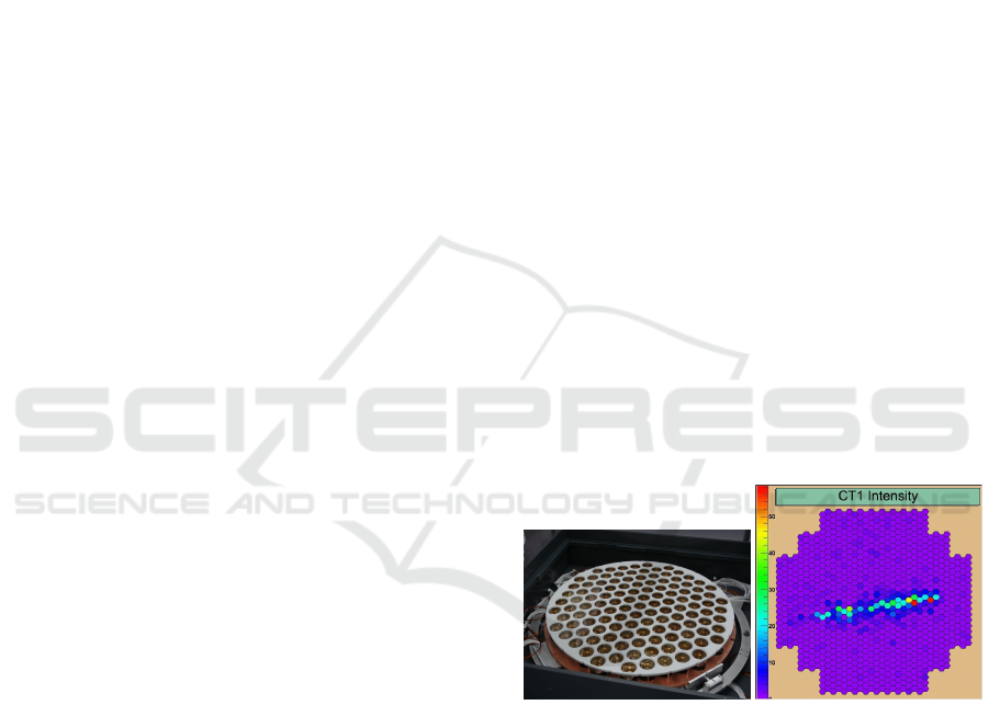
Figure 1: Example of physics experiments presenting non-
Cartesian sensor grids. On the left, the XENON1T photo-
multiplier tube layout. Credit: XENON Collaboration. On
the right, an image from the H.E.S.S. camera. Credit: The
H.E.S.S. collaboration.
spect the original layout of the images, like in Hex-
aConv (Hoogeboom et al., 2018). In this paper, the
authors present group convolutions for square pixels
and hexagonal pixel images. A group convolution
consists in applying several transformations (e.g. ro-
tation) to the convolution kernel to benefit from the
axis of symmetry of the images. In the hexagonal grid
case they use masked convolutions applied to hexago-
nal pixel images represented in the Cartesian grid (via
shifting).
362
Jacquemont, M., Antiga, L., Vuillaume, T., Silvestri, G., Benoit, A., Lambert, P. and Maurin, G.
Indexed Operations for Non-rectangular Lattices Applied to Convolutional Neural Networks.
DOI: 10.5220/0007364303620371
In Proceedings of the 14th International Joint Conference on Computer Vision, Imaging and Computer Graphics Theory and Applications (VISIGRAPP 2019), pages 362-371
ISBN: 978-989-758-354-4
Copyright
c
 2019 by SCITEPRESS – Science and Technology Publications, Lda. All rights reserved

However, such approaches may have several
drawbacks:
• oversampling or geometric transformation may
introduce distortions that can potentially result in
lower accuracy or unexpected results;
• oversampling or geometric transformation impose
additional processing, often performed at the CPU
level which slows inference in production;
• geometric transformation with masked convolu-
tion adds unnecessary computations as the mask
has to be applied to the convolution kernel at each
iteration;
• oversampling or geometric transformations can
change the image shape and size.
In order to prevent these issues and be able to work
on unaltered data, we present here a way to apply
convolution and pooling operators to any grid, given
that each pixel neighbor is known and provided. This
solution, denoted indexed operations in the follow-
ing, driven by scientific applications, is applied to an
hexagonal kernel since this is one of the most com-
mon lattice besides the Cartesian one. However, in-
dexed convolution and pooling are very general solu-
tions, easily applicable to other domains with irregu-
lar grids.
At first, a reminder of how convolution and pool-
ing work and are usually implemented is done. Then
we present our custom indexed kernels for convolu-
tion and pooling. This solution is then applied to stan-
dard datasets, namely CIFAR-10 and AID to validate
the approach and test performances. Finally, we dis-
cuss the results obtained as well as potential applica-
tions to real scientific use cases.
2 CONVOLUTION
2.1 Background
Convolution is a linear operation performed on data
over which neighborhood relationships between ele-
ments can be defined. The output of a convolution
operation is computed as a weighted sum (i.e. a dot
product) over input neighborhoods, where the weights
are reused over the whole input. The set of weights is
referred to as the convolution kernel. Any input data
can be vectorized and then a general definition of con-
volution can be defined as:
O
j
=
K
∑
k=1
w
k
I
N
jk
(1)
where K is the number of elements in the kernel, w
k
is the value of the k-th weight in the kernel, and N
jk
is the index of the k-th neighbor of the j-th neighbor-
hood.
This general formulation of discrete convolution
can be then made more specific for data over which
neighborhood relationships are inherent in the struc-
ture of the input, such as 1D (temporal), 2D (image)
and 3D (volumetric) data. For instance, in the case of
classical images with square pixels, we define convo-
lution as:
O
i j
=
W
∑
k=−W
H
∑
h=−H
w
kh
I
(i−k)( j−h)
(2)
where the convolution kernel is a square matrix of
size (2W + 1, 2H +1) and neighborhoods are implic-
itly defined through corresponding relative locations
from the center pixel. Analogous expressions can be
defined in N dimensions.
Since the kernel is constant over the input, i.e. its
values do not depend on the location over the input,
convolution is a linear operation. In addition, it has
the advantage of accounting for locality and transla-
tion invariance, i.e. output values solely depend on
input values in local neighborhoods, irrespective of
where in the input those values occur.
Convolution cannot be performed when part of the
neighborhood cannot be defined, such as at the bor-
der of an image. In this case, either the correspond-
ing value in the output is skipped, or neighborhoods
are extended beyond the reach of the input, which is
referred to as padding. Input values in the padded re-
gion can be set to zero, or reproduce the same values
as the closest neighbors in the input.
It is worth noting that the convolution can be com-
puted over a subset of the input elements. On reg-
ular lattices this results in choosing one every n ele-
ments in each direction, an amount generally referred
as stride. The larger the stride, the smaller the size of
the output.
The location of neighbors in convolution kernels
does not need to be adjacent, as it is in the image for-
mulation above. Following the first expression, neigh-
borhoods can be defined arbitrarily, in terms of shape
and location of the neighbors. In case of regular lat-
tices the amount of separation between the elements
of a convolution kernel in each direction is referred to
as dilation or atrous convolution (Holschneider et al.,
1990). The larger the dilation, the further away from
the center the kernel reaches out in the neighborhood.
In case of inputs with multiple channels such as an
RGB images, or multiple features in intermediate lay-
ers in a neural network, all input channels contribute
to the output and convolution is simply obtained as
the sum of dot products over all the individual chan-
nels to produce output values. Equation 3 shows the
Indexed Operations for Non-rectangular Lattices Applied to Convolutional Neural Networks
363

2D image convolution case with C input channels.
O
i j
=
C
∑
c=1
W
∑
k=−W
H
∑
h=−H
w
ckh
I
c(i−k)( j−h)
(3)
Therefore, the size of kernels along the channel di-
rection determines the number of input features that
the convolution operation expects, while the number
of individual kernels employed in a neural network
layer determines the number of features in the output.
2.2 Implementation
In neural network applications convolutions are per-
formed over small spatial neighborhoods (e.g. 3 × 3,
5 × 5 for 2D images). Given the small size of the el-
ements in the dot product, the most computationally
efficient strategy for computing the convolution is not
an explicitly nested loop as described on equation 2,
but a vectorized dot product over all neighborhoods.
Then, as most deep learning frameworks intensively
do, one can make use of the highly optimized ma-
trix multiplication operators available in linear alge-
bra libraries (van de Geijn and Goto, 2011). Let us
consider the im2col operation that transforms any in-
put (1D, 2D, 3D and so on) into a 2D matrix where
each column reports the values of the neighbors to
consider for each of the input samples (respectively,
time stamp, pixel, voxel and so on) as illustrated in the
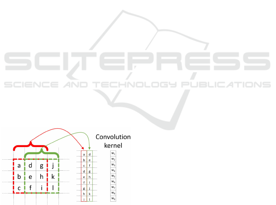
example given in figure 2. Given this layout, convolu-
tion consists in applying the dot product of each col-
umn with the corresponding flattened, columnar ar-
rangement of weights of the convolution kernel. Per-
forming the dot product operation over all neighbor-
hoods amounts to a matrix multiplication between the
column weights and the column image.
Figure 2: Example of pixel neigborghood arrangements for
a 3 × 3 kernel.
In multiple channel case (see equation 3 for C
input channels), all input channels contribute to the
output. At the column matrix level, this translates
into stacking individual columns from all channels
along a single column, and similarly for the kernel
weights. Conversely, in order to account for multi-
channel output, multiple column matrices are consid-
ered, or, equivalently, the column matrix and the cor-
responding kernel weights have an extra dimension
along C
out
.
In this setting, striding consists in applying the
im2col operation on a subset of the input, while di-
lation consists in building columns according to the
dilation factor, using non-immediate neighbors. Last,
padding can be achieved by adding zeros (or the
padded values of choice) along the columns of the
column matrix.
Owing to the opportunity for vectorization and
cache friendliness of the general matrix multiply op-
erations (GEMM), the resulting gains in efficiency
outweigh the additional memory consumption due to
duplication of values in the column image, since ev-
ery value in the input image will be replicated in as
many locations as the neighbors it participates to (see
figure 2).
The im2col operation is easily reversible. This
will be considered for deep neural networks training
steps where the backward gradient propagation is ap-
plied in order to optimize the network parameters.
3 INDEXED KERNELS
Given the general interpretation of convolution and its
implementation as given in the previous sections, the
extension of convolution from rectangular lattices to
more general arrangements is now straightforward.
Given an input vector of data and a matrix of
indices describing every neighborhood relationships
among the elements of the input vectors, a column
matrix is constructed by picking elements from the
input vector according to each neighborhood in the
matrix of indices. Analogously to the case of rect-
angular lattices, neighborhoods from different input
channels are concatenated along individual columns,
as are kernel weights. At this point, convolution can
be computed as a matrix multiplication.
We will now show how the above procedure can
be performed in a vectorized fashion by resorting to
advanced indexing. Modern multidimensional array
frameworks, such as NumPy, TensorFlow and Py-
Torch, implement advanced indexing, which consists
in indexing multidimensional arrays with other multi-
dimensional arrays of integer values. The integer ar-
rays provide the shape of the output and the indices
at which the output values must be picked out of the
input array.
In our case, we can use the matrix of indices de-
VISAPP 2019 - 14th International Conference on Computer Vision Theory and Applications
364

scribing neighborhoods in order to index into the in-
put tensor, producing the column matrix in one pass,
both on CPU and GPU devices. Since the indexing
operation is differentiable with respect to the input
(but not with respect to the indices), a deep learn-
ing framework equipped with automatic differenti-
ation capabilities (like PyTorch or TensorFlow) can
provide the backward pass automatically as needed.
We will now present a PyTorch implementation of
such indexed convolution in a hypothetical case.
We consider in the following example an input
tensor with shape B, C
in
, W
in
, where B is the batch size
equal to 1, C
in
is the number of channels equal to 2,
or features, and W
in
is the width equal to 5, i.e. the
number of elements per channel,
input = torch.ones(1, 2, 5)
and a specification of neighbors as an indices tensor
with shape K, W
out
, where K is the size of the con-
volution kernel equal to 3 and W
out
equal to 4 is the
number of elements per channel in the output
indices = torch.tensor([[ 0, 0, 3, 4],
[ 1, 2, 4, 0],
[ 2, 3, 0, 1]])
where values, arbitrarily chosen in this example, rep-
resent the indices of 4 neighborhoods of size 3 (i.e.
neighborhoods are laid out along columns). The num-
ber of columns corresponds to the number of neigh-
borhoods, i.e. dot products, that will be computed
during the matrix multiply, hence they correspond to
the size of the output per channel.
The weight tensor describing the convolution ker-
nels has shape [C
out
, C
in
, K], where C
out
equal to 3 is
the number of channels, or features, in the output. The
bias is a column vector of size C
out
.
weight = torch.ones(3, 2, 3)
bias = torch.zeros(3)
At this point we can proceed to use advanced in-
dexing to build the column matrix according to in-
dices.
col = input[..., indices]
Here we are indexing a B, C
in
, W
in
tensor with a
K, W
out
tensor, but the indexing operation has to pre-
serve batch and input channels dimensions. To this
end, we employ the ellipsis notation ..., which pre-
scribes indexing to be replicated over all dimensions
except the last. This operation produces a tensor
shaped B, C
in
, K, W
out
, i.e. 1, 2, 3, 4.
As noted above, the column matrix needs values
from neighborhoods for all input channels concate-
nated along individual columns. This is achieved by
reshaping the col tensor so that C
in
and K dimensions
are concatenated:
B = in pu t . sh ap e [ 0]
W_ ou t = i ndi ce s . sh ap e [1 ]
col = col . v ie w (B , -1 , W_ out )
The columns in the col tensor are now a concate-
nation of 3 values (the size of the kernel) per input
channel, resulting in a B, K · C
in
, W
out
. Note that the
col tensor is still organized in batches.
At this point, weights must be arranged so that
weights from different channels are concatenated
along columns as well:
C_ ou t = w eig ht . s hap e [0]
we ig ht _co l = we igh t . vie w ( C_o ut , -1)
which leads from a C
out
, C
in
, K to a C
out
, K ·C
in
ten-
sor.
Multiplying the weight_col and col matrices will
now perform the vectorized dot product correspond-
ing to the convolution:
out = to rch . mat mu l ( we i gh t_ co l , col )
Note that we are multiplying a C
out
, K ·C
in
tensor
by a B, K ·C
in
, W
out
tensor, to obtain a B, C
out
, W
out
ten-
sor. In this case, the B dimension has been automati-
cally broadcast, without extra allocations.
In case bias is used in the convolution, it must be
added to each element of the output, i.e. a constant is
summed to all values per output channel. In this case,
bias is a tensor of shape C
out
, so we can perform the
operation by again relying on broadcasting on the first
B and last W
out
dimension:
out += bias . u n squ e e z e (1)
Padding can be handled by prescribing a place-
holder value, e.g. −1, in the matrix of indices. The
following instruction shows an example of such a
strategy:
indices = torch.tensor([[-1, 0, 3, 4],
[ 1, 2, 4, 0],
[ 2, 3, 0, 1]])
The location can be used to set the corresponding
input to the zero padded value, though multiplication
of the input by a binary mask. Once the mask has been
computed, the placeholder can safely be replaced with
a valid index so that advanced indexing succeeds.
indices = indices.clone()
padded = indices == -1
indices[padded] = 0
mask = torch.tensor([1.0, 0.0])
mask = mask[..., padded.long()]
col = input[..., indices] * mask
Indexed Operations for Non-rectangular Lattices Applied to Convolutional Neural Networks
365

4 POOLING
4.1 Pooling Operation
In deep neural networks, convolutions are often asso-
ciated with pooling layers. They allow feature maps
down-sampling thus reducing the number of network
parameters and so the time of the computation. In ad-
dition, pooling improves feature detection robustness
by achieving spatial invariance (Scherer et al., 2010).
The pooling operation can be defined as:
O
i
= f (I
N
i
) (4)
where O
i
is the output pixel i, f a function, I
N
i
the
neighborhood of the input pixel i of a given input fea-
ture map I. The pooling function f provided on eq.
4 is applied on I
N
i
using a sliding window. f can be
of various forms, for example an average, a Softmax,
a convolution or a max. The use of a stride greater
than 2 on the sliding window translation enables to
sub-sample the data. With convolutional networks, a
max-pooling layer with stride 2 and width 3 is typi-
cally considered moving to a 2 times coarser feature
maps scale after having applied some standard con-
volution layers. This proved to reduce network over-
fit while improving task accuracy (Krizhevsky et al.,
2012).
4.2 Indexed Pooling
Following the same procedure as for convolution de-
scribed in section 3, we can use the matrix of indices
to produce the column matrix of the input and apply,
in one pass, the pooling function to each column.
For instance, a PyTorch implementation of the in-
dexed pooling, in the same hypothetical case as pre-
sented in section 3, with max as the pooling function
is:
col = input[..., indices]
out = torch.max(col, 2)
5 APPLICATION EXAMPLE: THE
HEXAGONAL CASE
The indexed convolution and pooling can be applied
to any pixel organization, as soon as one provides
the list of the neighbors of each pixel. Although
the method is generic, we first developed it to be
able to apply Deep Learning technic to the hexag-
onal grid images of the Cherenkov Telescope Ar-
ray (from NectarCam, Glicenstein et al. 2013; LST-
Cam, Ambrosi et al. 2013; and FlashCam, Pühlhofer
et al. 2012). Even if hexagonal data processing is
not usual for general public applications, several other
specific sensors make use of hexagonal sampling. The
Lytro light field camera (Cho et al., 2013) is a con-
sumer electronic device example. Several Physics ex-
periments also make use of hexagonal grid sensors,
such as the H.E.S.S. camera (Bolmont et al., 2014)
or the XENON1T detector (Scovell, 2013). Hexag-
onal lattice is also used for medical sensors, such as
DEPFET (Neeser et al., 2000) or retina implant sys-
tem (Schwarz et al., 1999).
Moreover, hexagonal lattice is a well-known and
studied grid (Sato et al., 2002; Shima et al., 2010;
Asharindavida et al., 2012; Hoogeboom et al., 2018)
and offers advantages compared to square lattice
(Middleton et al., 2001) such as higher sampling den-
sity and a better representation of curves. In addi-
tion, some more benefits have been shown by (Sousa,
2014; He and Jia, 2005; Asharindavida et al., 2012)
such as equidistant neighborhood, clearly defined
connectivity, smaller quantization error.
However, processing hexagonal lattice images
with standard deep learning frameworks requires spe-
cific data manipulation and computations that need to
be optimized on CPUs as well as GPUs. This sec-
tion proposes a method to efficiently handle hexago-
nal data without any preprocessing as a demonstration
of the use of indexed convolutions. We first describe
how to build the index matrix for hexagonal lattice
images needed by the indexed convolution.
For easy comparison, we want to validate our
methods on datasets with well-known use cases (e.g.
a classification task) and performances. To our
knowledge, there is no reference hexagonal image
dataset for deep learning. So, following Hexa-
Conv paper (Hoogeboom et al., 2018) we constructed
two datasets with hexagonal images based on well-
established square pixel image datasets dedicated to
classification tasks: CIFAR-10 and AID. This enables
our method to be compared with classical square pix-
els processing in a standardized way.
5.1 Indexing the Hexagonal Lattice and
the Neighbors’ Matrix
As described in section 3, in addition to the image
itself, one needs to feed the indexed convolution (or
pooling) with the list of the considered neighbors for
each pixel of interest, the matrix of indices. In the
case of images with a hexagonal grid, provided a
given pixel addressing system, a simple method to re-
trieve these neighbors is proposed.
Several addressing systems exist to handle images
with such lattice, among others: offset (Sousa, 2014),
VISAPP 2019 - 14th International Conference on Computer Vision Theory and Applications
366

ASA (Rummelt, 2010), HIP (Middleton et al., 2001),
axial - also named orthogonal or 2-axis obliques
(Asharindavida et al., 2012; Sousa, 2014). The latter
is complete, unique, convertible to and from Carte-
sian lattice and efficient (He and Jia, 2005). It offers a
straightforward conversion from hexagonal to Carte-
sian grid, stretching the converted image, as shown in
figure 3, but preserving the true neighborhood of the
pixels.
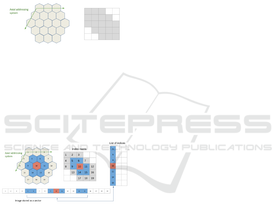
Figure 3: Hexagonal to Cartesian grid conversion with the
axial addressing system.
Our method relies on the axial addressing system
to build an index matrix of hexagonal grid images.
Assuming that a hexagonal image is stored as a vector
and that we have the indices of the pixels of the vec-
tor images represented in the hexagonal grid, one can
convert it to an index matrix thanks to the axial ad-
dressing system. Then, building the list of neighbors,
the matrix of indices, consists in applying the desired
kernel represented in the axial addressing system to
the index matrix for each pixel of interest.
Figure 4: Building the matrix of indices for an image with
a hexagonal grid. The image is stored as a vector, and the
indices of the vector are represented in the hexagonal lattice.
Thanks to the axial addressing system, this representation
is converted to a rectangular matrix, the index matrix. The
neighbors of each pixel of interest (in red) are retrieved by
applying the desired kernel (here the nearest neighbors in
the hexagonal lattice, in blue) to the index matrix.
An example is proposed on fig. 4, with the ker-
nel of the nearest neighbors in the hexagonal lattice.
Regarding the implementation, one has to define in
advance the kernel to use as a mask to be applied to
the index matrix, for the latter example:
kernel = [[1, 1, 0],
[1, 1, 1],
[0, 1, 1]]
5.2 Experiment on CIFAR-10
The indexed convolution method, in the special case
of hexagonal grid images, has been validated on the
CIFAR-10 dataset. For this experiment and the one
on the AID dataset (see Sec. 5.3), we compare our
results with the two baseline networks of HexaConv
paper (Hoogeboom et al., 2018). These networks do
not include group convolutions and are trained respec-
tively on square and hexagonal grid image versions
of CIFAR-10. The network trained on the hexagonal
grid CIFAR-10 consists of masked convolutions. To
allow a fair comparison, we use the same experimen-
tal conditions, except for the Deep Learning frame-
work and the square to hexagonal grid image trans-
formation of the datasets.
The CIFAR-10 dataset is composed of 60000 tiny
color images of size 32x32 with square pixels. Each
image is associated with the class of its foreground
object. This is one of the reference databases for im-
age classification tasks in the machine learning com-
munity. By converting this square pixel database into
its hexagonal pixel counterpart, this enables to com-
pare hexagonal and square pixel processing in differ-
ent case studies for image classification. This way,
the same network with:
• standard convolutions (square kernels),
• indexed convolutions (square kernels),
• indexed convolutions (hexagonal kernels),
has been trained and tested, respectively on the
dataset for the square kernels and its hexagonal ver-
sion for the hexagonal kernels. For reproducibility,
the experiment has been repeated 10 times with dif-
ferent weights initialization, but using the same ran-
dom seeds (i.e. same weights initialization values) for
all three implementations of the network.
5.2.1 Building a Hexagonal CIFAR-10 Dataset
The first step is to transform the dataset in a hexago-
nal one. Compared to a rectangular grid, an hexagonal
grid has one line out of two shifted of half a pixel (see
figure 5). Square pixels (orange grid) cannot be re-
arranged directly in a hexagonal grid (blue grid). For
these shifted lines, pixels have to be interpolated from
the integer position pixels of the rectangular grid. The
interpolation chosen here is the average of the two
consecutive horizontal pixels. A fancier method could
have been to take into account all the six square pix-
els contributing to the hexagonal one, in proportion
to their involved surface. In that case, the both pix-
els retained for our interpolation method would cover
90.4% of the surface of the interpolated hexagonal
pixel.
Indexed Operations for Non-rectangular Lattices Applied to Convolutional Neural Networks
367

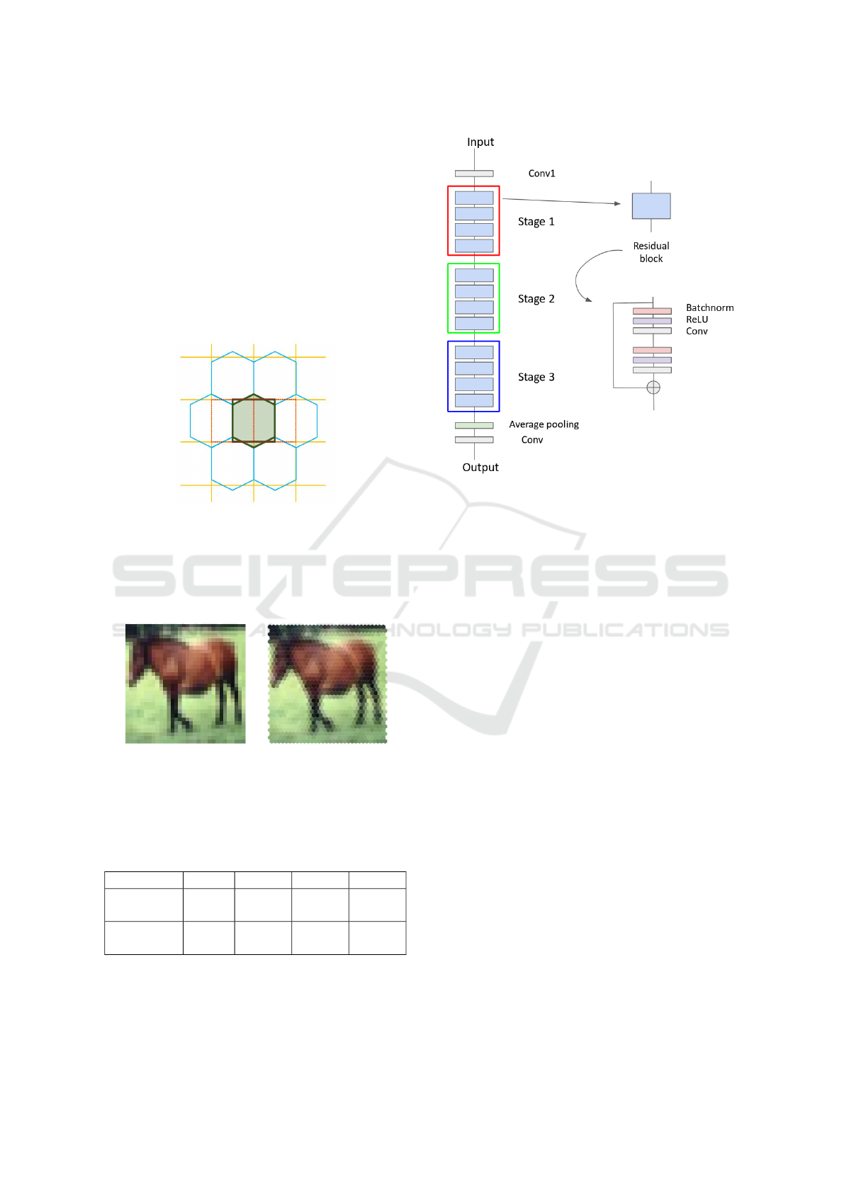
Fig. 6 shows a conversion example, one can ob-
serve that the interpolation method is rough as one can
see on the back legs of the horse so that hexagonal
processing experiments suffer from some input image
distortion. However, our preliminary experiments did
not show strong classification accuracy difference be-
tween such conversion and a higher quality one.
Then the images are stored as vectors and the in-
dex matrix based on the axial addressing system is
built. Before feeding the network, the images are
standardized and whitened using a PCA, following
Hoogeboom et al. 2018.
Figure 5: Resampling of rectangular grid (orange) images
to hexagonal grid one (blue). One line of two in the hexag-
onal lattice is shifted by half a pixel compared to the corre-
sponding line in the square lattice. The interpolated hexag-
onal pixel (with a green background) is the average of the
two corresponding square pixels (with red dashed borders).
Figure 6: Example of an image from CIFAR-10 dataset re-
sampled to hexagonal grid.
5.2.2 Network Model
Table 1: Number of features for all three hexagonal and
square networks used on CIFAR-10.
conv1 stage 1 stage 2 stage 3
Hexagonal
kernels
17 17 35 69
Square
kernels
15 15 31 61
The network used for this experiment is described
in section 5.1 of (Hoogeboom et al., 2018) and re-
lies on a ResNet architecture (He et al., 2015). As
shown in figure 7, it consists of a convolution, 3 stages
Figure 7: ResNet model used for the experiment on CIFAR-
10.
with 4 residual blocks each, a pooling layer and a
final convolution. The down-sampling between two
stages is achieved by a convolution of kernel size
1x1 and stride 2. After the last stage, feature maps
are squeezed to a single pixel (1x1 feature maps) by
the use of an average pooling over the whole feature
maps. Then a final 1x1 convolution (equivalent to a
fully connected layer) is applied to obtain the class
scores. Three networks have been implemented in Py-
Torch, one with built-in convolutions (square kernels)
and two with indexed convolutions (one with square
kernels and one with hexagonal kernels). Rectangular
grid image versions have convolution kernels of size
3x3 (9 pixels) while the one for hexagonal grid im-
ages has hexagonal convolution kernels of the nearest
neighbors (7 pixels). The number of features per layer
is set differently, as shown in table 1, depending on
the network so that the total number of parameters of
all three networks are close, ensuring the comparison
to be fair. These networks have been trained with the
stochastic gradient descent as optimizer with a mo-
mentum of 0.9, a weight decay of 0.001 and with a
learning rate of 0.05 decayed by 0.1 at epoch 50, 100
and 150 for a total of 300 epochs.
5.2.3 Results
As shown in table 2, all three networks with hexag-
onal indexed convolutions, square indexed convolu-
tions and square standard convolutions exhibit simi-
lar performances on the CIFAR-10 dataset. The dif-
VISAPP 2019 - 14th International Conference on Computer Vision Theory and Applications
368

ference between the hexagonal kernel and the square
kernel with standard convolution on the one hand and
between both square kernel is not significant, accord-
ing to the Student T test. For the same number of
parameters, the hexagonal kernel model gives slightly
better accuracy than the square kernel one in the con-
text of indexed convolution, even if the images have
been roughly interpolated for hexagonal image pro-
cessing. However, to satisfy this equivalence in the
number of parameters, since hexagonal convolutions
involve fewer neighbors than the squared counterpart,
some more neurons are added all along the network
architecture. This leads to a larger number of data
representations that are combined to achieve the task.
One can then say that Hexagonal convolution pro-
vides richer features for the same price in the param-
eters count. This may also compensate for the im-
age distortions introduced when converting input im-
ages to hexagonal sampling. Such distortions actually
sat Hexagonal processing in an unfavourable initial
state but the hexagonal processing compensated and
slightly outperformed the standard approach.
Hoogeboom et al. (2018) carried out a similar ex-
periment and observed the same accuracy difference
between hexagonal and square convolutions process-
ing despite a shift in the absolute accuracy values
(88.75 for hexagonal images, 88.5 for square ones)
that can be explained by different image interpolation
methods, different weights initialization and the use
of different frameworks.
Table 2: Accuracy results for all three hexagonal and square
networks on CIFAR-10. i. c. stands for indexed convolu-
tions.
Hexagonal
kernels (i.c.)
Square
kernels (i.c.)
Square
kernels
88.51 ± 0.21 88.27 ± 0.23 88.39 ± 0.48
5.3 Experiment on AID
Similar to the experiment on CIFAR-10, the indexed
convolution has been validated on Aerial Images
Dataset (AID) (Xia et al., 2016). The AID dataset
consists of 10000 RGB images of size 600x600
within 30 classes of aerial scene type. Similar to
section 5.2, the same network with standard convo-
lutions (square kernels) and then with indexed convo-
lutions (square kernels and hexagonal kernels) have
been trained and tested, respectively on the dataset
for the square kernels and its hexagonal version for
the hexagonal kernels. The experiment has also been
repeated ten times, but with the same network ini-
tialization and different random split between train-
ing set and validating set, following Hoogeboom et al.
(2018).
5.3.1 Building a Hexagonal AID Dataset
After resizing the images to 64x64 pixels, the dataset
is transformed to a hexagonal one, as shown fig. 8, in
the same way as in section 5.2.1. Then the images are
standardized.
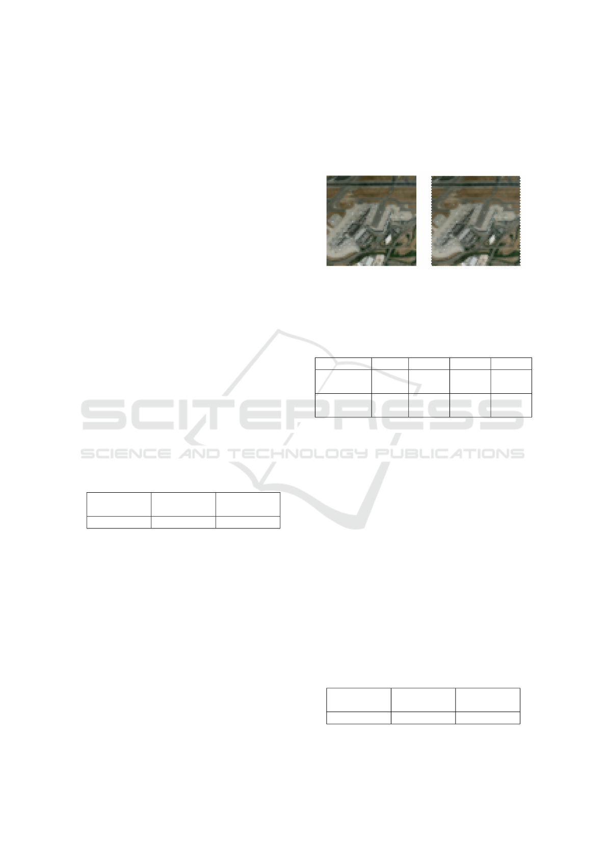
Figure 8: Example of an image from AID dataset resized
to 64x64 pixels and resampled to hexagonal grid.
5.3.2 Network
Table 3: Number of features for all three hexagonal and
square networks used on AID.
conv1 stage 1 stage 2 stage 3
Hexagonal
kernels
42 42 83 166
Square
kernels
37 37 74 146
The network considered in this experiment is still
a ResNet architecture but adapted to this specific
dataset. One follows the setup proposed in section 5.2
of Hoogeboom et al. 2018. Three networks have been
implemented and trained in the same way described
in section 5.2.2, with the number of features per layer
described in table 3.
5.3.3 Results
As shown in table 4, all three networks with hexago-
nal convolutions and square convolutions do not ex-
hibit a significant difference in performances on the
AID dataset. Again, no accuracy loss is observed in
the hexagonal processing case study despite the rough
image re-sampling.
However, unlike on the CIFAR-10 experiment, we
don’t observe a better accuracy of the model with
hexagonal kernels, as emphasized in (Hoogeboom
et al., 2018).
Table 4: Accuracy results for all three hexagonal and square
networks on AID. i. c. stands for indexed convolutions.
Hexagonal
kernels (i.c.)
Square
kernels (i.c.)
Square
kernels
79.81 ± 0.73 79.88 ± 0.82 79.85 ± 0.50
Indexed Operations for Non-rectangular Lattices Applied to Convolutional Neural Networks
369

6 COMMENTS/DISCUSSION
This paper introduces indexed convolution and pool-
ing operators for images presenting pixels arranged
in non-Cartesian lattices. These operators have been
validated on standard images as well as on the special
case of hexagonal lattice images, exhibiting similar
performances as standard convolutions and therefore
showing that the indexed convolution works as ex-
pected. However, the indexed method is much more
general and can be applied to any grid of data, en-
abling unconventional image representation to be ad-
dressed without any pre-processing. This differs from
other approaches such as image re-sampling com-
bined with masked convolutions (Hoogeboom et al.,
2018) or oversampling to square lattice (Holch et al.,
2017) that actually require additional pre-processing.
Moreover, both methods increase the size of the trans-
formed image (adding useless pixels of padding value
for the resampled image to be rectangular and / or
multiplying the number of existing pixels) and are re-
stricted to regular grids. On the other hand, they make
use of out the box operators already available in cur-
rent deep learning frameworks.
The approach proposed in this paper is not lim-
ited to hexagonal lattice and only needs the index
matrices to be built prior the training and inference
processes, one for each convolution of different in-
put size. No additional pre-processing of the image
is then required to apply convolution and pooling ker-
nels. However, the current implementation in Python
shows a decrease in computing performances com-
pared to the convolution method implemented in Py-
torch. We have observed an increase of RAM usage of
factors varying between 1 and 3 and training times of
factors varying between 4 and 8 on GPU (depending
on the GPU model), of factor 1.5 on CPU (but slightly
faster than masked convolutions on CPU) depending
on the network used.
These drawbacks are actually related to the use of
un-optimized codes and work is carried out to fix this
by the use of optimized CUDA and C++ implementa-
tions.
As a future work, we will use the indexed oper-
ations for the analysis of hexagonal grid images of
CTA. We also plan to experiment with arbitrary ker-
nels, which are another benefit of the indexed opera-
tions, for the convolution (e.g. retina like kernel with
more density in the center, see the example in the
github repository).
ACKNOWLEDGEMENTS
This project has received funding from the European
Union’s Horizon 2020 research and innovation pro-
gram under grant agreement No 653477.
This work has been done thanks to the facilities of-
fered by the Université Savoie Mont Blanc MUST
computing center.
REFERENCES
Ambrosi, G., Awane, Y., Baba, H., et al. (2013). The
cherenkov telescope array large size telescope. arXiv
preprint arXiv:1307.4565.
Asharindavida, F., Hundewale, N., and Aljahdali, S. (2012).
Study on hexagonal grid in image processing. 45:282–
288.
Bolmont, J., Corona, P., Gauron, P., et al. (2014). The
camera of the fifth h.e.s.s. telescope. part i: System
description. Nuclear Instruments and Methods in
Physics Research Section A: Accelerators, Spectrom-
eters, Detectors and Associated Equipment, 761:46 –
57.
Cho, D., Lee, M., Kim, S., and Tai, Y.-W. (2013). Modeling
the calibration pipeline of the lytro camera for high
quality light-field image reconstruction. In Proceed-
ings of the IEEE International Conference on Com-
puter Vision, pages 3280–3287.
Glicenstein, J., Barcelo, M., Barrio, J., et al. (2013). The
NectarCAM camera project. ArXiv e-prints.
He, K., Zhang, X., Ren, S., and Sun, J. (2015). Deep
residual learning for image recognition. CoRR,
abs/1512.03385.
He, X. and Jia, W. (2005). Hexagonal structure for intelli-
gent vision. In Information and Communication Tech-
nologies, 2005. ICICT 2005. First International Con-
ference on, pages 52–64. IEEE.
Holch, T. L., Shilon, I., Büchele, M., et al. (2017). Probing
convolutional neural networks for event reconstruc-
tion in gamma-ray astronomy with cherenkov tele-
scopes. arXiv preprint arXiv:1711.06298.
Holschneider, M., Kronland-Martinet, R., Morlet, J., and
Tchamitchian, P. (1990). A real-time algorithm for
signal analysis with the help of the wavelet transform.
In Combes, J.-M., Grossmann, A., and Tchamitchian,
P., editors, Wavelets, pages 286–297, Berlin, Heidel-
berg. Springer Berlin Heidelberg.
Hoogeboom, E., Peters, J. W., Cohen, T. S., and Welling,
M. (2018). Hexaconv. In International Conference on
Learning Representations.
Katz, U. (2012). A neutrino telescope deep in the Mediter-
ranean Sea. CERN Cour., 52N6:31–33.
Krizhevsky, A., Sutskever, I., and Hinton, G. E. (2012). Im-
agenet classification with deep convolutional neural
networks. In Advances in neural information process-
ing systems, pages 1097–1105.
VISAPP 2019 - 14th International Conference on Computer Vision Theory and Applications
370

Middleton, L., Sivaswamy, J., and Coghill, G. (2001). The
fft in a hexagonalimage processing framework. New
Zealand Conference on Image and Vision Computing
(IVCNZ 2001), (January):231–236.
Neeser, W., Bocker, M., Buchholz, P., et al. (2000). The
depfet pixel bioscope. IEEE Transactions on Nuclear
Science, 47(3):1246–1250.
Pühlhofer, G., Bauer, C., Biland, A., et al. (2012). Flash-
Cam: A fully digital camera for CTA telescopes. In
Aharonian, F. A., Hofmann, W., and Rieger, F. M., ed-
itors, American Institute of Physics Conference Series,
volume 1505 of American Institute of Physics Confer-
ence Series, pages 777–780.
Rummelt, N. I. (2010). Array set addressing: enabling effi-
cient hexagonally sampled image processing. Univer-
sity of Florida.
Sato, H., Matsuoka, H., Onozawa, A., and Kitazawa, H.
(2002). Hexagonal image representation for 3-d pho-
torealistic reconstruction. In Pattern Recognition,
2002. Proceedings. 16th International Conference on,
volume 2, pages 672–676. IEEE.
Scherer, D., Müller, A., and Behnke, S. (2010). Evaluation
of pooling operations in convolutional architectures
for object recognition. In Artificial Neural Networks–
ICANN 2010, pages 92–101. Springer.
Schwarz, M., Hauschild, R., Hosticka, B. J., et al. (1999).
Single-chip cmos image sensors for a retina implant
system. IEEE Transactions on Circuits and Systems
II: Analog and Digital Signal Processing, 46(7):870–
877.
Scovell, P. (2013). The Xenon 100 Detector. In Cline, D.,
editor, Springer Proceedings in Physics, volume 148
of Springer Proceedings in Physics, page 87.
Shima, T., Sugimoto, S., and Okutomi, M. (2010). Com-
parison of image alignment on hexagonal and square
lattices. In Image Processing (ICIP), 2010 17th IEEE
International Conference on, pages 141–144. IEEE.
Sousa, N. A. (2014). Hexagonal grid image processing al-
gorithms in neural vision and prediction. pages 1–19.
van de Geijn, R. and Goto, K. (2011). BLAS (Basic Linear
Algebra Subprograms), pages 157–164. Springer US,
Boston, MA.
Xia, G., Hu, J., Hu, F., et al. (2016). AID: A benchmark
dataset for performance evaluation of aerial scene
classification. CoRR, abs/1608.05167.
Indexed Operations for Non-rectangular Lattices Applied to Convolutional Neural Networks
371